Chapter 4 Accessibility and Deception

4.1 Summary

This chapter will discuss how we can improve the accessibility of our data visualisations for diverse audiences. This not only includes people with a vision impairment, but also many other types a disability that ultimately impacts a person’s ability to engage with digital content. Ensuring that our designs are more widely accessible will increase their reach and overall effectiveness. This chapter also takes a close look at some of the most common methods used in data visualisation that risk deception, real or perceived, and useful strategies for minimising this risk in your own work.

4.1.1 Acknowledgements

I would like to acknowledge the contributions of my former students, Roshana Rahgozar, Kieu Chinh Vu, Campbell Timms, Bhavika Shrestha and Hrishika Kaur Arora for assisting with the development of the accessibility section of this chapter. Their research, ideas, thoughtful discussion and feedback helped immensely in shaping this important, and long-overdue, course topic. I must also thank Dr. Ronny Andrade Parra, accessibility guru, for encouraging me to develop this topic and drawing my attention to the fabulous work of Elavsky, Bennett, and Moritz (2022).

4.1.2 Learning Objectives

The learning objectives for this chapter are as follows:

• Discuss the importance of accessibility in data visualisation design by referring to common access issues experienced by people with disability.
• Describe the most common types of assistive technologies used by people with disability to access digital content.
• Discuss the principles of accessible design for data visualisation and the ongoing challenges facing the field.
• Identify and address common data visualisation accessibility issues using a range of practical methods.
• Identify and discuss the following deceptive data visualisation issues:
  • The issue with pie and doughnut charts
  • Truncated axes
  • Using area or size to depict a quantity
  • Changing plot aspect ratio
  • Ignoring convention
  • Dual axes
  • Other poor scaling methods
  • Visual bombardment
• Discuss and apply practical strategies for avoiding the deceptions above.

4.2 Improving accessibility

Accessibility within the context of data visualisation can be defined simply as the practice of maximising diverse audience engagement, interaction and understanding (Elavsky, n.d.). Designers must be able to identify and, ultimately, mitigate accessibility barriers (Elavsky, Bennett, and Moritz 2022). As you will discover, this is by no means an easy task. The goal of this section is to develop a fundamental understanding of common barriers and some practical solutions to design more accessible data visualisations. You will also learn where to find more detailed information and discuss the challenges that remain. Firstly, let’s consider the reasons why accessibility matters and introduce the guiding principles of accessible design.

The World Wide Web Consortium (2024) Web Content Accessibility Guidelines 2.2 (WCAG 2.2) are a good place to start to help understand accessibility as it relates to data visualisation. Most data visualisations these days, and media in general, are published on the web or via apps. WCAG 2.2 aims to help web and app developers make their content more accessible to people with a range of different disabilities such as the following:

• Blindness and vision impairment
• Deafness and hearing loss
• Movement limitations
• Speech impairment
• Photosensitivity
• And, to a limited extent, learning and cognitive limitations

A sizable proportion of the general population will have one or more of these disabilities so improving the accessibility of web content and other digital technologies can help increase the audience and improve the experience for many. For example, in 2018, 1 in 6 (18%) of Australians were estimated to be living with a disability and this prevalence drastically increases to 50% for people aged 65 or over (Australian Institute of Health and Welfare 2024a). Note that these figures include all types of disabilities. If we look specifically at conditions which impact vision, prevalance remains very high.

According to the National Health Survey of 2022 (Australian Bureau of Statistics 2023), approximately 14 million, or 1:2, Australians self-report at least one chronic eye condition. Table 4.1 (Australian Bureau of Statistics 2023) reports the types of conditions and their estimated prevalence in the Australian population for 2022. Conditions vary in terms of the challenges they present to the individual with more severe conditions, such as blindness (full and partial), macular degeneration and cataracts being less common. More prevalent conditions, such as hyperopia, myopia, astigmatism and presbyopia have effective interventions such a corrective lenses and surgery. Regardless, conditions that impact vision are highly prevalent, not only in Australia, but the rest of the world.

Table 4.1: National Health Survey, 2022, Estimated diseases of the eye and adnexa, all persons (Australian Bureau of Statistics 2023)

Condition	Persons ’000	Appox. odds
Long sighted / hyperopia	7730.3	1:3
Short sighted / myopia	7152.0	1:4
Astigmatism	1859.6	1:14
Other diseases of the eye and adnexa	964.0	1:26
Presbyopia	735.5	1:34
Cataract	563.7	1:45
Colour blind	537.4	1:48
Macular degeneration	263.4	1:100
Glaucoma	221.7	1:111
Blindness (complete and partial)	154.6	1:167
Total diseases of the eye and adnexa	14422.1	1:2

It is also important to note that eye conditions, and disability more broadly, don’t impact everyone equally. For example, women and elderly people are at higher risk of experiencing chronic eyes conditions according to Figure 4.1 which was published by Australian Institute of Health and Welfare (2021) using ABS data. Furthermore, Aboriginal and Torres Strait Islander people are at higher risk when compared to nonindigenous Australians (Australian Institute of Health and Welfare 2024b). The type of eye condition also depends on factors such as age and sex. For example, men are far more likely to have colour blindness, 4% versus 0.3% for women.

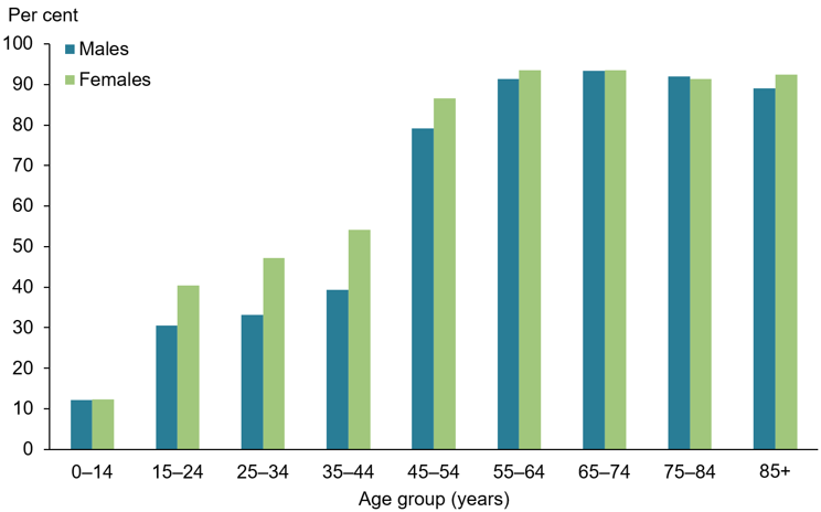
Figure 4.1: This clustered bar chart taken from Australian Institute of Health and Welfare (2021) and based on ABS 2019 National Health Survey data shows the increased prevalence (%) of chronic eye conditions (plotted on the y-axis) in women and the elderly. Prior to 45, women have much higher rates compared to men. However, after 45, rates for both sexes almost double from about 40% to 80% by the age of 54 and the gap between men and women closes. This chart has been copied directly from Australian Institute of Health and Welfare (2021) under a Creative Commons BY 4.0 licence.

Accessibility issues in data visualisation are not only limited to conditions that impact vision. The Center for Accessibility Australia (2024) provides a list of the common online content access issues for people with different forms of disability. The list has been directly quoted from Center for Accessibility Australia (2024), specifically the page “How will people with disability engage with my content?” click here.

Vision For people who are blind or vision impaired, common accessibility issues include:

• The inability for screen readers to process images;
• Poor colour contrast;
• Colour being used by itself to indicate a change;
• Lack of audio description in videos;
• Links that lack description such as ‘click here’ or ‘read more’
• Missing or incorrect heading labels
• Poor navigation structure

Hearing For people who are Deaf or hearing impaired, common accessibility issues include:

• Lack of captions in video;
• Lack of transcripts for audio-only content such as podcasts;
• Lack of sign language
• Use of audio by itself to indicate a change or an action

Mobility For people with a mobility impairment, common accessibility issues include:

• Content auto-refreshing without any mechanism to slow down or stop the process;
• A mistaken selection is made in a drop-down menu and the user is instantly taken to the incorrect selection;
• Speech navigation software does not work correctly due to missing labels;
• Content requires precise movement of a mouse to operate

Cognitive For people with a cognitive impairment, common accessibility issues include:

• Confusing layout
• Poorly labelled form fields;
• Menus and links not working in a predictable way
• Lack of definition for abbreviations and acronyms;
• Lack of an Easy English summary sheet;

As you have read, accessibility in data visualisation extends beyond conditions that impact vision. For example, many cognitive limitations impact memory which will limit the amount of information that people can hold, manipulate and recall. Executive function and processing speed might also be limited meaning that extra support and time for interpreting visualisations may be required. Fine motor skills decrease as we age making the operation of many everyday technologies like computer mice and touch screens more difficult to use.

People with disability adapt as best they can in order to access everyday technologies that many of us take for granted. For example, people with blindness or low vision will use a range of assistive technologies such as screen magnifiers, themes that adjust colours and the size of onscreen elements and screen readers. According to Vision Australia (2024) the most common screen readers used by their clients were Apple’s VoiceOver, Job Access with Speech (JAWS), NVDA, Microsoft Narrator and Google TalkBack. Screen readers are used to read digital text and metadata back to users to help them navigate, operate and access information on their devices. They are often controlled by keyboards, so keyboard compatibility and testing are important. Studies suggest that screen reader access to data visualisations remains very poor. For example, Fan et al. (2023) found from an audit of 76 top Google ranked COVID-19 related data visualisations that the vast majority had very poor screen reader compatibility. Therefore, data visualisation designers have lots of room for improvement.

4.2.1 Accessibility principles for data visualisation

Designers need a set of guiding principles to enhance accessibility. The Web Content Accessibility Guidelines (WCAG, developed by the Web Accessibility Initiative) provides a useful starting point (World Wide Web Consortium 2024). The WCAG principles, abbreviated as POUR, are quoted and defined as follows:

• Perceivable: Information and user interface components must be presentable to users in ways they can perceive.
• Operable: User interface components and navigation must be operable.
• Understandable: Information and the operation of the user interface must be understandable.
• Robust: Maximize compatibility with current and future user agents, including assistive technologies.

Elavsky, Bennett, and Moritz (2022) extended POUR and added the three additional principles: (c)omprising, (a)ssistive and (f)lexible (CAF), to make POUR-CAF. POUR-CAF was targeted at the specific design needs of data visualisation.

CAF can briefly defined as follows:

• Compromising: Designs accommodate for different means in which users prefer to consume digital information including the use of assistive technologies.
• Assistive: Designs reduce functional and cognitive loads so that the audience can gain value from the visualisation.
• Flexible: Designs must be capable of adapting to user needs and preferences.

Elavsky, Bennett, and Moritz (2022) used these principles to develop a data visualisation accessibility evaluation tool, which they named Chartability.The current version of the Chartability Workbook available on Github details 50 heuristics of which 14 are considered critical to address (Elavsky 2025). A heuristic in this context is defined as a testable question that relates to accessibility. A full audit would test all 50 heuristics, track failures and make recommendations. Elavsky reports that a complete audit can take anywhere between 2 to 8 hours depending on the visualisation. This isn’t practical in most situations and certainly not when learning the foundations of data visualisation. The following sections won’t teach you how to undertake a full audit (this requires specialised training). Instead, they aim to help designers better identify common accessibility issues related to data visualisation and provide some practical strategies on how to minimise them.

4.2.2 Practical accessibility

The following sections discuss how designers can improve the accessibility of their data visualisations. Figure 4.2 show a heatmap by Dattani and Spooner (2025) that will be used as an example to aid the discussion. The heatmap shows the effect of vaccines on measles prevalence across time in the US. This was published following a serious measles outbreak during 2022 in the US that originated in Texas and spread to surrounding states (“2025 Southwest United States Measles Outbreak” 2026). The objective was to remind the audience that vaccines are the most effective preventative tool for controlling the spread of serious infectious diseases. The outbreak in the US was largely attributed to increased rates of vaccine exemptions sought for children in kindergarten and early schooling.

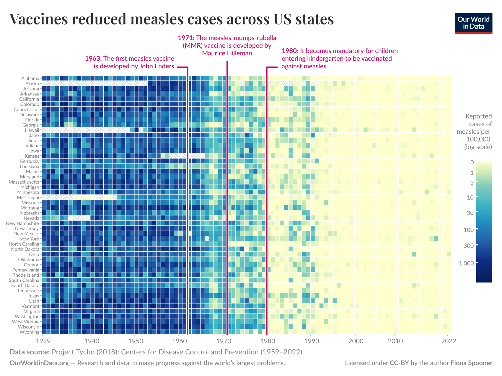
Figure 4.2: This heatmap shows the reported cases of measles per 100,000 of the population using a log scale across time (x-axis, Yearly, 1929 - 2022) and US states (y-axis). Log cases are encoded using a continuous colour scale that ranges from light beige (0 cases) to a dark blue (1000+ cases). The heat map includes annotations for 1963 when the first measles vaccine was developed by John Enders and later in 1971 with the measles-mumps-rubella (MMR) vaccine by Maurice Hilleman. A final annotation highlighting 1980 marks the time at which the US made vaccination mandatory (Dattani and Spooner 2025).

The heatmap in Figure 4.2 is a great example of a high information data visualisation with narrative components. The reliance on colour, text, and small visual elements present some interesting accessibility challenges to help contextualise the following discussion.

4.2.3 Alt support

📝 Note

• Use descriptive titles, subtitles, captions and other text to support visuals.
• Ensure alt text is available for screen readers.
• Ensure font size isn’t too small.
• Consider alt formats.

Our data visualisations should be supported by non-graphical, or alternative (“alt” for short), components beyond axis labels and scale legends. This typically refers to the addition of descriptive text such as titles, subtitles and captions. This is a simple and highly effective way to improve accessibility. Text can be read alongside the data visualisaiton to help the audience understand and focus on the key insights. It can also be used in place of the visuals if the data visualisation cannot be seen (i.e. due to blindness or for technical reasons). There are lots of considerations regarding the effective use of alt support that we need to understand. Let’s start by considering what textual support is recommended for each data visualisation.

Evergreen and Emery (2016) have already provided a helpful checklist of how to use text appropriately for data visualisation. Despite this checklist not being focused specifically on accessibility, it is a great starting point. Here is a list of the “Text” aspect guidelines proposed by Evergreen and Emery (2016):

• 6-12 word descriptive title is left-justified in upper left corner
• Subtitle and/or annotations provide additional information
• Text size is hierarchical and readable
• Text is horizontal
• Data are labeled directly
• Labels are used sparingly

As you can see, most of these recommendations will help with accessibility. The checklist starts with the inclusion of a descriptive title that includes a key take-away message. This can be a sentence that captures the “so what?” question of a graph. Subtitles can add further detail and context about the graph and data. Looking back to Figure 4.2, we note the inclusion of a short descriptive title, “Vaccines reduced measles cases across US states”. There was no subtitle, but there was lots of accompanying annotations and labels which build up a clear picture of the data and main insights. However, as the data visualisation is presented using a bitmap image, this text must be read from the image. What happens if you can’t see the text in the image?

People with low vision or blindness often rely on screen reader technology that typically cannot access text embedded in images. Extracting text from images would require the use of a generative model or optical character recognition (OCR) technology. This is a computationally expensive and much slower process that reading digital text. This is why WCAG 2.2 requires the use of “alt” text for all important graphical content published on the web. The “alt” attribute is used in HTML to attach a textual description to an image. Screen readers are designed to access this “alt” text. Figure 4.3 shows how to find a web data visualisation’s “alt” text using the Inspect tool in Microsoft Edge.

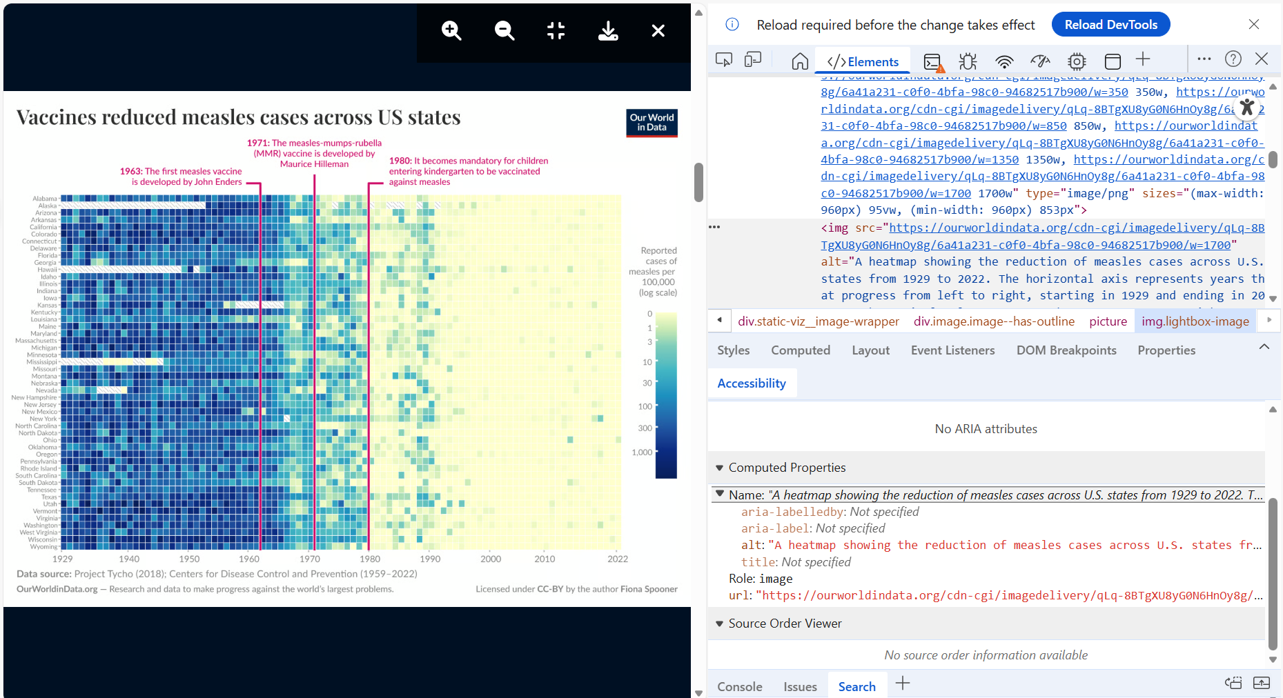
Figure 4.3: Inspecting the webpage code of the measles vaccine heatmap by Dattani and Spooner (2025) introduced back in Figure 4.2 reveals the presence of an alternative, “alt” text attribute, which screenreaders rely on.

Extracting the “alt” text from Dattani and Spooner (2025), we find a helpful and detailed textual summary as follows:

<img src="https://ourworldindata.org/cdn-cgi/imagedelivery/qLq-8BTgXU8yG0N6HnOy8g/6a41a231-
c0f0-4bfa-98c0-94682517b900/w=1700" alt="A heatmap showing the reduction of measles cases 
across U.S. states from 1929 to 2022. The horizontal axis represents years that progress 
from left to right, starting in 1929 and ending in 2022. Each vertical column corresponds 
to a U.S. state, with states labeled on the left side. The colors in each cell represent 
the number of reported measles cases per 100,000 people, using a logarithmic scale. Darker 
shades of blue indicate higher numbers of cases, while lighter shades transition to yellow,
signifying fewer cases. 

Key historical milestones are marked with vertical lines and text: 
- 1963 indicates the development of the first measles vaccine by John Enders.
- 1971 highlights the introduction of the measles-mumps-rubella (MMR) vaccine by Maurice 
Hilleman.
- 1980 notes that vaccination becomes mandatory for children entering kindergarten.

At the bottom, a data source citation credits Project Tycho (2018) and the Centers for Disease 
Control and Prevention (1959–2022). There’s additional attribution to Our World in Data, which 
focuses on global progress against major issues. The work is licensed under CC-BY by the author 
Fiona Spooner." class="lightbox-image" loading="lazy" width="1700" height="1276">

Adding a detailed description of a data visualisation as a caption and also into the “alt” text is often overlooked. The extra time and effort to do so might explain why. However, its important for accessibility. Cleveland (1994) lists three essential components of a good data visualiaation description (p. 55):

1. Describe everything that is graphed.
2. Draw attention to the important features of the data.
3. Describe the conclusions that are drawn from the data on the graph.

Looking back at the alt text extracted from Dattani and Spooner (2025), 1. and 2. have been done very well. However, 3. is overlooked. Dattani and Spooner (2025) should add something along the lines of the following:

Since the first introduction of the measles vaccine in 1963 and the MMR vaccine later in 1971, measles cases across all US states declined drastically. Law reform in 1980 requiring children entering the schooling system to be vaccinated furthered this decline. From the mid 1990s to 2020s, measles cases have remained negligable. While, outbreaks have occured during this time, vaccines have contained spead and outbreak duration. Vaccines remain the most effective way to prevent the spread of measles.

Font size in another important consideration. Setting and checking the font size of textual elements within a data visualisation can be challenging and gets quite technical (see World Wide Web Consortium (2025) for a detailed discussion). This is because font size has a physical relationship to the display on which it is shown (Think about variability in screen sizes and pixel densities) Don’t trust your data visualisation tools either. Many tools and packages will scale font in order to fit titles and labels, avoid overlap or avoid breaking text across lines. Specify font sizes using your tool as best you can, but check the result and make refinements as required. A font size of 12px/9pt is considered the minimum. Reading font below this size becomes increasingly difficult for most people, not just those with a vision impairment. Therefore, we should use the highest possible font size that we can get away with, subject to the following constraints:

• Visuals first, text second
• Different font sizes are needed to represent hierarchy - E.g. Title, subtitle, labels/annotations.
• Avoid textual overlapping
• Text should be horizontal - avoid diagonal and vertical text

Check that your web browser is at 100% zoom and pay attention to the smaller fonts in your texual hierarchy. Use your commonsense. If you are having issues reading the font size of text, odds are it is too small. If you want to know how small, a simple way to estimate the font size is by comparing it known font sizes. Mozilla provides a simple website (click here) listing various font sizes. If you align this website to you visualisation you can quickly estimate a font size (see Figure 4.4).

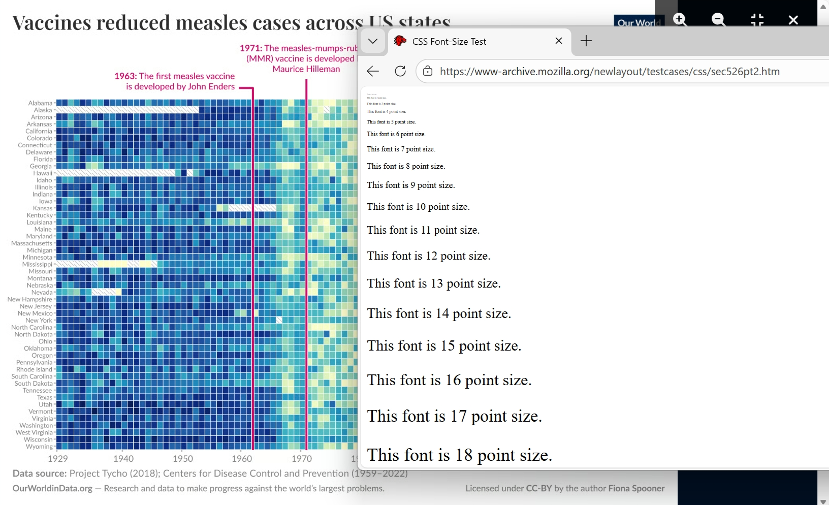
Figure 4.4: Comparing the font size used in the measles vaccine heatmap by Dattani and Spooner (2025) introduced back in Figure 4.2 to known font sizes is a quick way to find your smallest font size. The state labels used on the y-axis appear to have font size of 7-8pt. This is below the recommended minimum of 9pt. Therefore, we can expect many people to have difficulty reading the state labels on the y-axis without magnification.

What can you do if your font is too small? Simple. Find a way to increase it. This will depend largely on the nature of the data visualisation and the constraints under which you are working. Here are some ideas:

• Increase the size of the plot, horizontally, vertically or overall so there is more space to use larger font sizes
• Change the orientation of the plot to better fit textual components (e.g. change a bar plot from vertical to horizontal to accommodate longer textual labels)
• Abbreviate text ensuring you provide explanations in your caption/notes or by adding interactivity to provide full details.
• Remove redundant textual components to free up space - e.g. repeated legends, excessive labeling of axis tick marks
• Re-code categorical and ordinal variables to reduce the overall number of textual labels needed to be displayed. This must be done with caution so as not to change the story behind the data or hide important insights.
• Use interactivity to manage the display of textual information based on user preferences.

If your font is on the smaller size and you have done your best to maximise font size, warn your audience that zooming maybe required and ensure your visualisation is zoomable (high resolution).

You might also consider including alternate formats. For example, you may include a data table which can be read using a screenreader or interrogated by a generative model. You might also considering including an option to play an audio description. There is also some interesting research and tools based on sonification (Nees and Walker 2007; Flowers 2005; Brown et al. 2003), or turning data into sound. For example, Noisycharts (Evershed 2024) can add a sound layer to basic javascript plots. Figure 4.5 embeds an example taken from Evershed (2024).

Figure 4.5: This line chart is an example of a Noisychart provided by Evershed (2024). Press the “play” button to hear the data.

4.2.4 Magnification

📝 Note

• Publish using high resolution bitmap images or scalable vector graphics that maintain acuity on magnification.

Visual impairment often results in decreased visual acuity or the ability to see in detail. This ranges in severity based on the underlying condition, but even minor drops in acuity can substantially impact the experience of the viewer. Magnifying or “zooming” is a technological way in which people can manage low visual acuity. By bending light (magnification) or re-scaling/stretching an image on a digital display (digital zooming), the viewer can bring the image closer to observe in better detail. Therefore, a simple way to improve accessibility is to ensure that our data visualisations have sufficient resolution to support magnification. This prevents graphical and textual components within data visualisations from becoming blurry or excessively pixelated. Cheap high density displays, fast internet connections and cheap web storage means creating and displaying high quality graphics has never been easier. However, best not to assume anything and it is quick to check.

Check your data visualisations for potential issues with magnification by zooming in to 200% (see Figure 4.6. Ensure graphical and textual components remain sharp and focused. If pixelation is apparent or text looks blurry (go back and check font size to), you need to increase the image resolution using your data visualisation tool. Most tools allow you to export or scale data visualisation at varying resolutions.

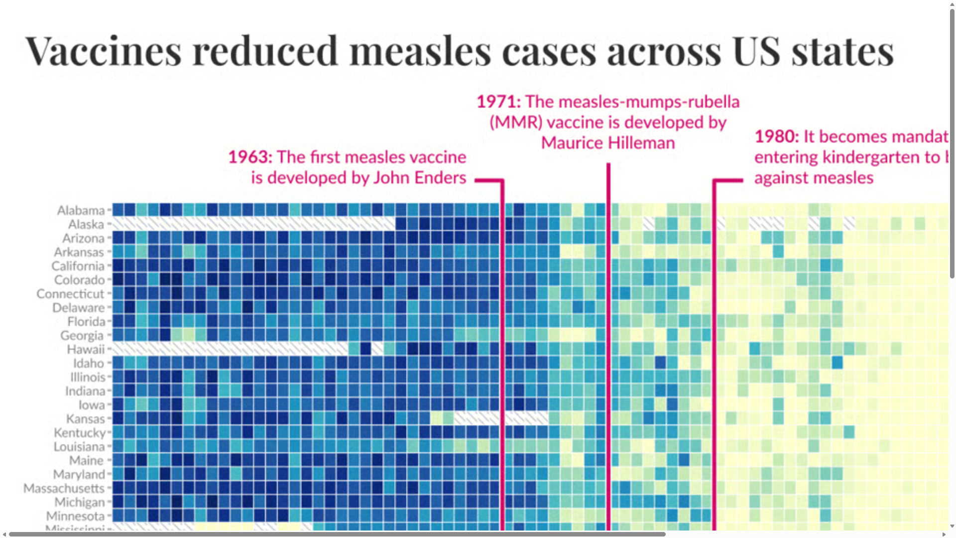
Figure 4.6: This figure shows 200% magnification of the vaccine heatmap by Dattani and Spooner (2025) introduced back in Figure 4.2. Text and graphical components remain sharp and focused at 200%.

Data visualisation tools based on Javascript often use scalable vector graphics (SVG) instead of bitmap. Bitmap images are based on grids of individual pixels that are coloured to create an image. SVG instead use web markup language to create images using mathematical models based on coordinate geometry. These models draw basic geometric shapes on a screen. Because graphics are stored as models, they can be easily “scaled” to the user. Figure 4.7 compares bitmap (raster) and SVG images. Bitmap images will eventually pixelate with progressive zooming. Pixelation appears much sooner with lower resolution images. SVG will never pixelate unless it is converted to a bitmap. If you are in the increasingly rare situation when you need to print a data visualisation, pay attention to your print DPI, or dots per square inch. 300DPI is considered the minimum (Ganner et al. 2023).

Figure 4.7: This figure by Yug and Cfaerber (2006) from Wikimedia Commons compares a bitmap image (raster) to SVG. SVG are infinitely scalable as they retain their sharpness because they are based on mathematical models that are drawn directly on the screen.

Furthermore, while it is true that data visualisations can be shrunk way down and retain their effectiveness (Tufte 2001), keep in mind that this might create issues with magnification. This is especially relevant for data visualisations that employ faceting or the use of small multiples (Faceting will be discussed in later chapters). Faceting relies on Tufte’s observation. However, ensuring the data visualisation has adequate resolution or the use of SVG will permit the audience to zoom when required without its potential drawbacks.

4.2.5 Contrast

📝 Note

• Text and graphical components must be adequately contrasted from the background.
• Pick colour scales that maximise contrast to the background and within the scale itself.
• Consider applying the “no use of colour alone” principle by adding redundant encodings, alt text, and interactivity.

Many people with visual impairments have decreased contrast sensitivity. Contrast in data visualisation is important because it allows our audience to differentiate the various graphical and textual components that make up a visualisation. Inadequate contrast is by far the most common accessibility issue raised during auditing according to Elavsky, Bennett, and Moritz (2022). Therefore, pay careful attention to contrast.

Contrast is discussed in terms of ratios. For example, the highest possible contrast can be found between black and white which has a contrast ratio of 21:1. You can read all about how this ratio is calculated if you are interested (click here). This is why a white background is so useful. It helps to maximise contrast with minimal effort.

According to the World Wide Web Consortium (2024) regular text needs a minimum contrast of 4.5:1. Larger text that might be used for a title can get away with 3:1. The geometric components of data visualisations including lines, points, bars and other geometric objects should also aim for 3:1 (Elavsky 2025). The primary focus here is between each colour used to convey information in the data visualisation and the background colour. All colours need adequate contrast from their background. Ensuring all colours have adequate contrast to each other quickly becomes impossible. For example, a colour scale with five different colours requires you to maintain a 3:1 ratio for 10 unique colour combinations (\({}^5C_2 = 10\)). As Kroes (2021) explains, this is impossible. The maximum number of colours that can maintain a 3:1 contrast ratio is 3! You can prove this using the Contrast Grid tool (click here). As Kroes writes:

If you are aiming for a minimum contrast of 3.0:1 between shades, then there can be only 3. You’ve got black at 1. Your shade at (at least) 3.0:1. And the next shade would be at (at least) 9.0:1. Because 9.0 has a contrast of 3.0:1 to 3.0. But, you can’t triple 9.0 once again. Then you’d get 27. And 27 is more than 21. You can’t create something brighter than white.

A compromise would be to check the contrast of colours that only share boundaries or overlap. That will often be difficult to check without missing certain combinations and the combinations will likely exceed three. What to do? We will discuss this further shortly, but for now let’s first focus our attention on background contrast.

How do we check it? There are many free online contrast checkers such as the following:

• WebAIM Contrast Checker - https://webaim.org/resources/contrastchecker/
• Cooler Contrast Check - https://coolors.co/contrast-checker
• Adobe Color Contrast Tool - https://color.adobe.com/create/color-contrast-analyzer

WebAIM and Cooler require you to input two colour codes (HEX, RGBm, etc) to calculate a ratio. If you don’t know the codes, you need to select them from the data visualisation using a colour picker. Adobe Color Contrast Tools allows you to upload an image of your data visualisation and pick two individual colours to contrast. However, each combination must be check using the same process. Upload, pick and contrast. This isn’t fun if you have lots of colours to check.

The Colour Contrast Analyser (CCA) by Vispero is completely free and much more powerful. It does require installation (PC and Mac are supported), but it makes it quicker and easier to check for contrast issues. The video in Figure 4.8 shows how to use CCA to isolate text and graphical colour codes and calculate contrast ratios based on the background. The video uses the measles vaccine heatmap by Dattani and Spooner (2025) introduced back in Figure 4.2. The animation shows the user selecting the text used to label each state on the y-axis. The text, which appears as a gray colour on a white background, lacks adequate contrast at 2.3:1. This fails WCAG requirements for small text. CCA can be used for everything displayed on your screen which makes it incredibly versatile and its provides a magnified view to easily isolate the colours of individual pixels. The output calculates the contrast ratio and tells you if you meet different WCAG guidelines. There are many other tools available, most are targeted at web design, that do a similar or better job, but which generally charge a subscription to access their full features.

Figure 4.8: This video shows how to use Colour Contrast Analyser, CCA, by Vispero to isolate text and graphical colour codes and calculate contrast ratios based on the background. The video uses the measles vaccine heatmap by Dattani and Spooner (2025) introduced back in Figure 4.2. The animation shows the user selecting the text used to label each state on the y-axis. The text, which appears as a gray colour on a white background, lacks adequate contrast at 2.3:1.

What about the contrast of colour scales used to represent different categories or quantitative values? For example, is the colour scale used to represent the log reported cases of measles per ’000 in Dattani and Spooner (2025)’s heatmap accessible? Absolutely not. No continuous colour scale will ever be considered accessible from a contrast standpoint. How could we possibly contrast between all colours on a continuum? Cleveland and McGill (1985) has already shown back in Chapter ?? that colour scales used for quantitative variables lack substantial accuracy. Sighted individuals with no visual impairments are only capable of distinguishing between and remembering a limited number of colours. For categorical or discrete colour scales MacDonald (1999) recommended a limit of only 5 - 7 colours. We have also discovered the uncomfortable truth that only three colours can be used if we want to maintain a contrast ratio of 3:1. How can a data visualisation designer’s favourite tool, colour, be such a problem for accessiblity?

Elavsky (2023) discusses this very problem in detail. While the traditional literature has focused on contrast as it relates to people with colour vision efficiency, less attention and consideration has been given to people with other types of visual impairment or people with lesser known conditions such as contrast sensitivity (see Irlen Syndrome). Elavsky recommends “no use of colour alone”, which requires redundancy of visual encoding. For example, colours representing groups are used in conjunction with texture. Points in a scatter plot representing different classes are displayed by colour and shape. There is no doubt that redundancy can help solve the colour contrast problem, but the resulting data visualisations often appear odd. For example, Figure 4.9 shows an accessible bar chart published by Elavsky (2023) which uses a redundant group encoding. Groups 1, 2 and 3 are encoded using both colour and texture (pattern). Yes, it is more accessible, but I don’t recommend the use of textures or patterns to achieve this.

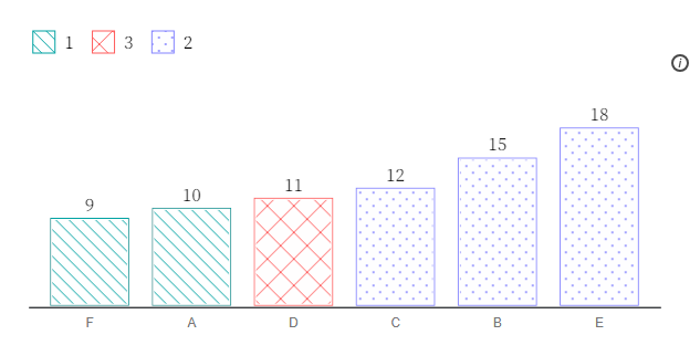
Figure 4.9: This figure shows an accessible bar chart published by Elavsky (2023) which uses a redundant group encoding. Groups 1, 2 and 3 are encoded using both colour and texture (pattern).

Tufte (2001) wrote extensively about moiré effects that can be created when textures appear to move or vibrate. This can cause visual stress and distract the audience. To quote Tufte in relation to the use of textures and their moiré effects:

“It is a clever idea, but no good examples are to be found. The key difficulty remains: moiré vibration is an undisciplined ambiguity, with an illusive, eye-straining quality that contaminates the entire graphic. It has no place in data graphical design.” (p. 112)

Tufte had very strong views on the use of texture in data visualisation, but texture is just one way that we can add redundancy to a graph. For example, facets can be used to replace both the need of colour and texture in the bar chart provided by Elavsky (2023) (see Figure 4.10.

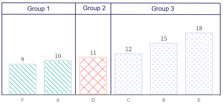
Figure 4.10: This figure shows the accessible bar chart published by Elavsky (2023) introduced back in Figure 4.9. By adding facets, there are now three ways to identify Groups 1, 2 and 3: panel, colour and texture (pattern). This is a triple encoding. However, both colour and texture can be removed without loss of information. Facets, or breaking a visualisation up into to smaller panels proves very accessible in this situation.

Many studies since have investigated the effect of redundancy used in data visualisation and the results range from being neutral to positive in terms of efficiency and accuracy (Jin et al. 2025; Chun 2017). However, many of these studies don’t deal specifically with the objective of improving accessibility. So there is still a lot of work to be done. We also need to keep in mind, that redundancy uses up a type of encoding that might better serve another purpose such as mapping an additional variable for deeper visual insight. Perhaps in time, Elavsky (2023)’s “no use of colour alone” will become accepted practice. I’m certainly open this to idea, but we need to be careful how we achieve it. I can’t see texture/pattern making a big comeback anytime soon.

4.2.6 Colour

📝 Note

• Use colour scales perceivable by people with colour vision deficiencies (avoid red-green)

We have dealt with the issue of contrasting textual and graphical components from their background. Colour plays a key role in contrast, however, there is also another common accessibility issue related to colour vision. Not all people perceive colour the same way. Colour vision deficiency (CVD), also referred to as colour blindness, is caused by missing or dysfunctional cones in the eye’s retina. The typical, “trichromatic” eye has three primary cones that detect the three primary colours of human vision, red, green and blue. If one or more of these cone types doesn’t work correctly or is missing, this is referred to as anomalous trichromacy. This is just a technical terms for someone with CVD. According to the National Health Survey of 2022 (Australian Bureau of Statistics 2023) there are an estimated 537,000 (2.1%) Australians living with CVD. The rates are much higher in men at 4% versus 0.3% for women. There are many variations based on the type and number of dysfunctional or missing cones in the retina. The green-red CVD types (deuteranopia and protanopia) are the most common. These types make it difficult to distinguish green and red. Figure 4.11, taken from Digital NSW (2023), will help you to understand the major classifications of CVD.

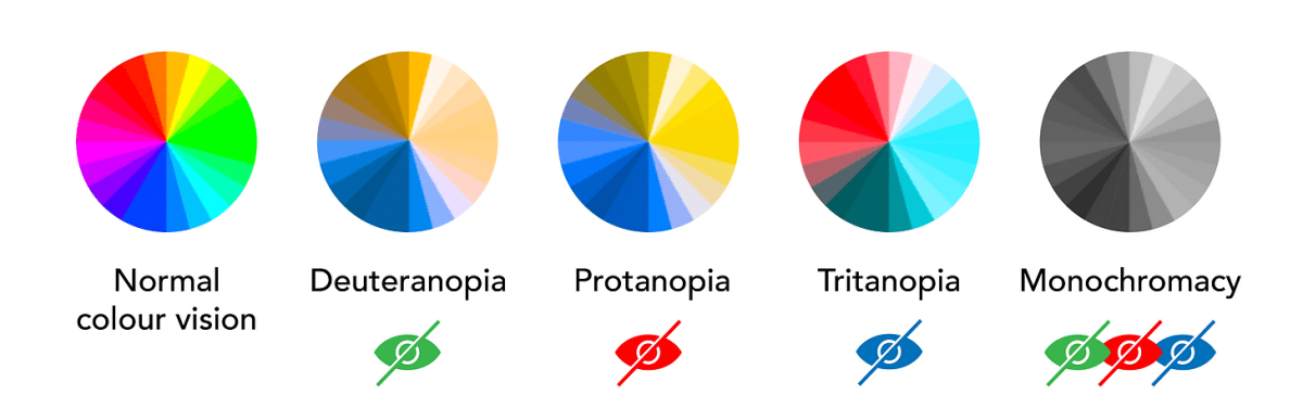
Figure 4.11: This figure was copied from Digital NSW (2023) under a Creative Commons Attribution 4.0 License. The figure visualises the differences between the major types of colour vision deficiency (CVD), namely deuteranopia, protanopia, tritanopia and monochromacy.

CVD can be partial or full. Deuteranopia refers to an inability to detect green, while deuteranomaly refers to reduced green sensitivity. Likewise, protanopia means no red vision, while protanomaly refers to a red insensitivity. These green-red CVD types make up the vast majority of CVD cases. Tritanopa and monochromacy are very rare. Therefore, from a practical accessibility standpoint, we really need to avoid colour scales that are based on red-green combinations.

Figure 4.12 shows how different types of CVD impact perceptions of colour (simulated). The images in Figure 4.12 were created using the Coblis Colour Blindness Simulator (Wickline 2001) and the choropleth map from the ColorBrewer web tool (Brewer and Harrower 2019).

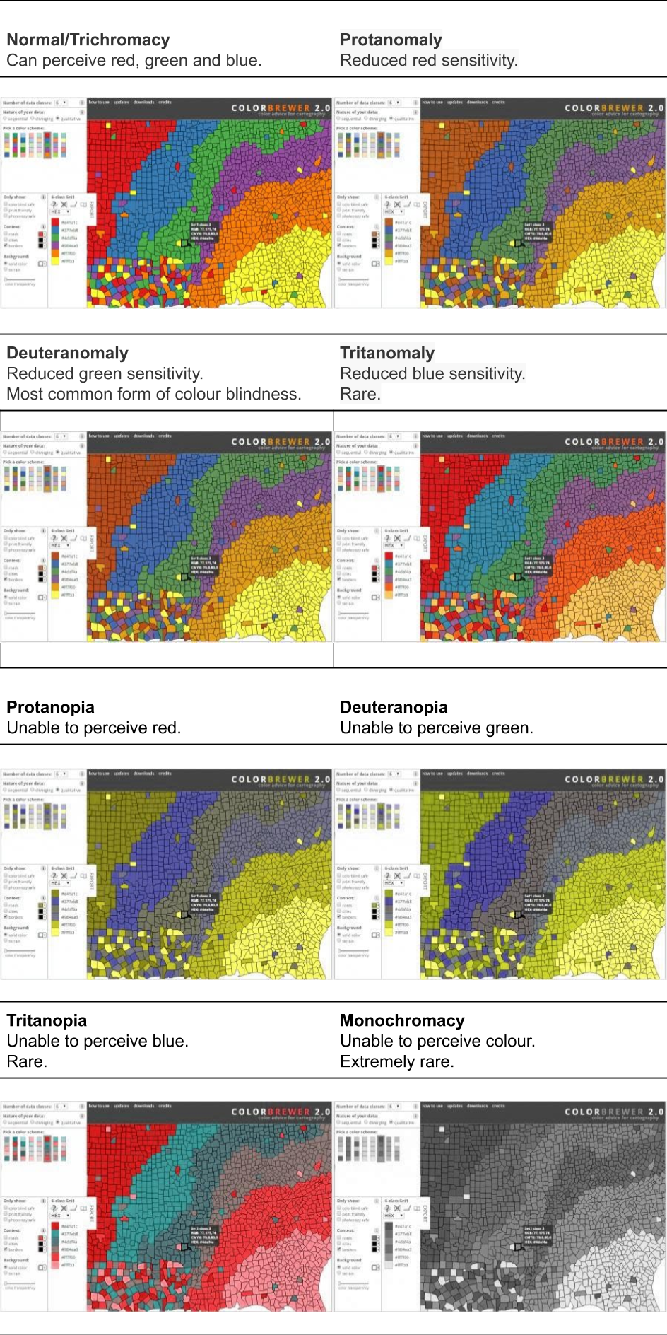
Figure 4.12: This figure shows how different types of CVD impact perceptions of colour (simulated). The images above were created using the Coblis Colour Blindness Simulator (Wickline 2001) and the choropleth map from the ColorBrewer web tool (Brewer and Harrower 2019).

CVD simulators can help us to predict how our data visualisation will appear to people with different types of CVD. There are many free tools available online. I recommend the Coblis Color Blindness Simulator (https://www.color-blindness.com/coblis-color-blindness-simulator/) which was used to create Figure 4.12. Focus on deuteranopia and protanopia if you are unsure about the CVD accessibility of a colour scale.

Using “off the shelf” colour palettes designed specifically for use in CVD populations is recommended, however, not always possible (e.g. if you are required to use a corporate colour palette). If you have the choice, the following colour palettes or schemes are recommended:

• ColorBrewer (Brewer and Harrower 2019) - https://colorbrewer2.org/
• Viridis (Garnier et al. 2024) - https://sjmgarnier.github.io/viridis/index.html
• Colour Universal Design (Okabe and Ito 2008) - https://jfly.uni-koeln.de/color/ (see https://easystats.github.io/see/reference/scale_color_okabeito.html for CUD R package)

Each of these colour scales can be implemented in all data visualisation tools by copying the appropriate colour codes or by using dedicated functions available for most open source tools.

4.2.7 Cognitive load

📝 Note

• Minimise distraction
• Write accessibly (consider reading level)
• Define abbreviations and technical terms
• Respect working memory limits

Cognitive barriers can be minimised in a number of ways. This means that our data visualisations allow our audience to focus on the important graphical insights and to not become distracted. Audiences can become distracted or overwhelmed by excessive text in the plot area, inclusion of images, bold grid lines, logos etc. We might also have to adjust our storytelling to slow down information, or build better scaffolding of our insights to enhance our audience’s understanding. This is where it pays to get feedback audience to help make refinements.

Write in an accessible manner. Think “plain English” here. Again, seek feedback from your audience and test their understanding. Ensure abbreviations and technical terms are defined clearly or references are provided to other sources that can help the audience. Ensure you help the audience to understand the main insights. Be explicit. Don’t assume everyone will “see” the insight, literally and figuratively. Audience understanding will be enhanced when multiple modes of communication (visual, written and verbal) work together.

Lastly, respect the limits of human working memory. For example, in relation to colour, we have already mentioned that MacDonald (1999) recommends 5 colours and 7 as an absolute maximum. However, Cowan (2010)’s review of the working memory research literature concluded that young adults can be expected to remember 3 - 5 chunks of information. A colour association can be thought of as a chunk. This capacity is lower in children, the elderly and many people with a cognitive impairment. This is why using intuitive colour associations can be so helpful. If an audience has learnt something like “Blue = Political Party A” or “blue - red = cold - hot”, the colour associations are readily retrieved from long-term memory. This also means that you should avoid using counter-intuitive associations or associations that require an audience to “unlearn”. For example, “blue = hot” and “red = cold” is counter-intuitive. Some colours are deeply ingrained in history, culture, education and branding. For example, in Australian politics, “Red = Labour”, “Blue = Liberals” and “Green = Greens”. If you change these associations, you are asking the audience to unlearn. Unlearning is harder than learning a new association. Using intuitive colour associations decreases cognitive load and makes interpretation of colour more efficient for all those that can that perceive it.

4.2.8 Assistive technology

📝 Note

• Ensure visualisations are screen reader ready
• Ensure interactive visualisations are keyboard compatible

Screen readers are one of the most common types of assistive technologies used by people with significant vision impairment. Previously, we discussed the importance of adding alt text to images of data visualisations so screen readers can “read” textual descriptions. It is also something worth experiencing and checking. You can load up your data visualisation using a popular screen reader to start checking. Common screen readers mentioned previously include the following:

• VoiceOver - https://www.apple.com/au/accessibility/vision/
• Job Access with Speech (JAWS) - https://www.freedomscientific.com/products/software/jaws/
• NVDA - https://www.nvaccess.org/download/
• Microsoft Narrator - https://www.microsoft.com/en-us/windows/tips/narrator
• Google TalkBack - https://belonging.google/intl/ALL_us/accessible-features/

This involves “keyboard probing” (Elavsky, Bennett, and Moritz 2022) or using common keys to navigate, search and select information on a screen. Take note of what information the screen reader reveals. Most importantly, can it read the data visualisation’s alt text? Can it find alt formats such as data tables or audio summaries? The compatibility between screen readers and data visualisations published on the web is generally poor (Fan et al. 2023), so do your best not to add to the problem.

Things get harder when we consider interactive data visualisations that require users to interact using computer inputs. Most online digital content is designed to be interacted with using touch screens and computer mice (and alternatives). However, for many people with disability, the trusty, but clunky, keyboard is the primary input device. Screen readers are designed carefully for keyboard compatibility as mice and touch screens rely heavily on sight (to locate the mouse pointer and where to touch).

Checking keyboard compatibility of interactive data visualisations is easy enough. Load up your interactive data visualisation in your web browser and start playing around with common keys. Take note of how the arrow keys move between inputs. Can the keys be used intuitively to select inputs, change options and update plots? What visual cues are present to help viewers track keyboard changes and select the appropriate input? Test common keys including arrow keys, tab, space, enter and escape. Ensure instructions are provided for keyboard users (You can read more here - https://webaim.org/techniques/keyboard/). You will probably discover issues, but fixing them goes well beyond the scope of this chapter.

Many interactive data visualisation tools are built to run in web browsers using a combination of web technologies including JavaScript, HTML and CSS. Therefore, they generally respond to keyboard inputs “out of the box”. However, somethings might not work as intended or require lengthy, unintuitive, and inefficient input. Fixing these problems gets very technical and will require customisation of the underlying code that drives the interactivity. This is where you might need to seek the assistance of an experienced web developer or allow extra time during the build to learn to fix these issues yourself. This is often well beyond the ability of someone learning data visualisation and even for most experienced designers.

4.2.9 Accessibility summary

The way that people experience the world can vary substantially from individual to individual. Sometimes the difference is stark, as can be the case for many people living with disability, but most of the time the consistency in the perceptive experience of our audience is remarkably similar. These shared experiences and how we consistently produce them, even when the data and context change, is the basis of good design. However, we also needs to be more accommodating and willing learn how to make our designs more accessible. The previous sections have shown that disability, which can result in many challenges with accessing digital content, is more common than you think. Design principles that guide the development of more accessible online content, including data visualisations, have been developed as a result. These principles aim to raise awareness of and break down common access barriers. This section has focused on many practical ways in which designers can improve the accessibility of their designs. However, challenges remain. Designing for accessibility is often limited by the tools and technology commonly used for data visualisation. Accessibility, unfortunately, is often an afterthought. Improvements are often ad-hoc and driven by the user community (Elavsky, Bennett, and Moritz 2022). These efforts have made an impact, but much work remains. We must continue to strive for better accessibility which will benefit all.

4.3 Avoiding deception

Intentional or not, data visualisations can obfuscate and deceive your audience (Bresciani and Eppler 2008). As Kirk (2012) reminds us, one of the four guiding principles of data visualisation is to avoid deception. According to Pandey et al. (2015) a deceptive data visualisation can be defined as follows:

a graphical depiction of information, designed with or without an intent to deceive, that may create a belief about the message and/or its components, which varies from the actual message” (p. 1471).

This definition ignores intent, which Kirk (2014) takes issue with. Kirk reasons that deception implies a deliberate attempt to mislead the audience. When the intent is not there, for example the designer is blissfully ignorant of the issue, the data visualisation is said to be confusing. This is semantically true, but the audience is rarely in a position to judge intent and, ultimately, the designer is responsible for their work. Therefore, if you do not take precautions, poor decisions can lead to a “perception of deception”. Data visualisation designers don’t get their day in court to judge intent, so you need to take reasonable steps to minimise this risk. Do not expect your audience to be as objective as Kirk (2014). Therefore, this next section will take a close look at some of the most common methods used in data visualisation that risk deception, real or perceived, and useful strategies for minimising this risk in your own work.

4.3.1 Pies and Doughnuts

Pie charts, and variations thereof, including the equally delicious doughnuts chart, are arguably the most controversial data visualisation ever created. Credited to the work of William Playfair, pie charts are now over 200 years old (Spence 2005). Love them or hate them, they are here to stay. So, why are pie charts so controversial? Should you use them? Are there better alternatives? The following section will explain.

Pie charts, and variations such as the doughnuts charts, are very common. You don’t need to trawl the internet or popular press for very long to find many examples. Energy Australia published a typical example of a pie chart, shown in Figure 4.13, which shows the market penetration of different forms of heaters in Australian in 2014 (Energy Rating 2019). This is a “good” example of a pie chart. Good use of colour, not too many categories, and labels and values included.

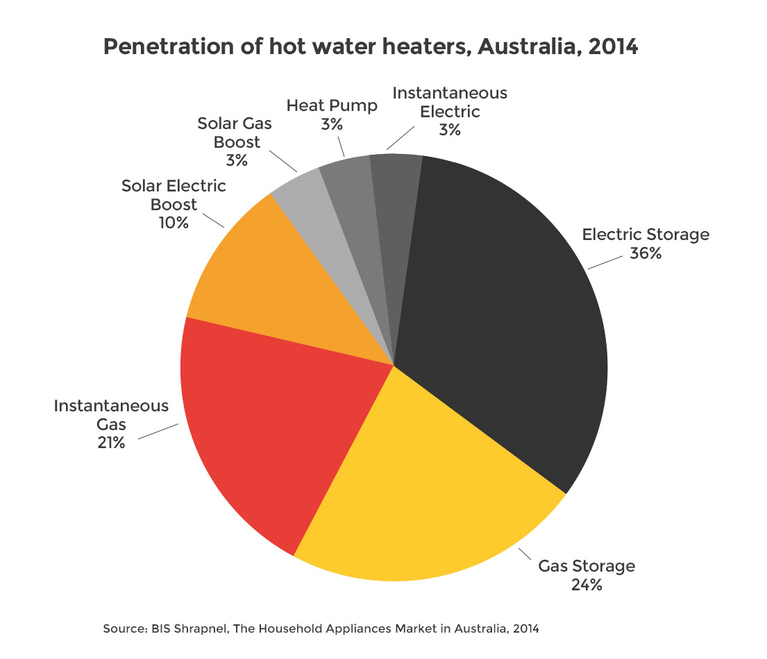
Figure 4.13: A typical pie chart (Energy Rating 2019).

Pie charts use angle to represent proportions or percentages. In Figure 4.14, the audience is forced to compare angle A to B. This is not an easy task to do accurately. Lucky for the value labels.

Figure 4.14: Pie charts require the comparison of angles (Energy Rating 2019).

Pie and doughnut charts also use area (see Figure 4.15). The viewer has to compare the area of each pie or doughnut slice. Skau and Kosara (2016) found that the most important aesthetic used in the interpretation of pie charts was area. So, the use of angle in pie charts isn’t the primary visual variable. Again, differences are easier to see when they are large, however, things get tricky when the proportions are similar.

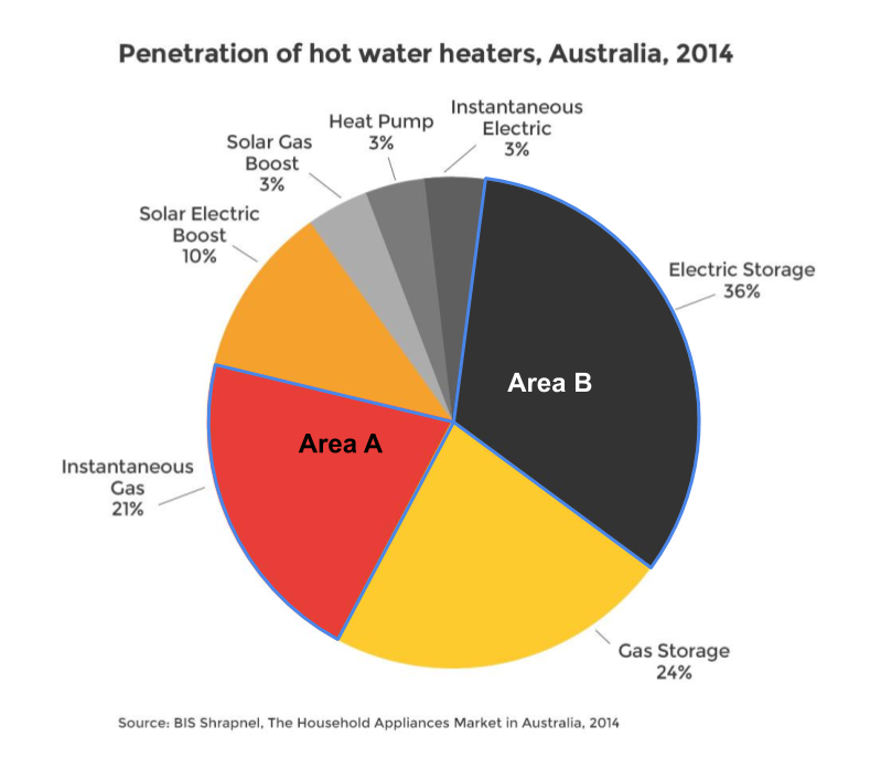
Figure 4.15: Pie charts also require comparison of area (Energy Rating 2019).

Figure 4.16 shows another example by Stanton and Alcorn (2016) from The Citizen. The pie charts are used to compare Australian emissions by state and then by industry for Victoria. They use the same colour scale to represent both state and economic sector which makes looking back and forth between the legend and pie charts very time consuming.

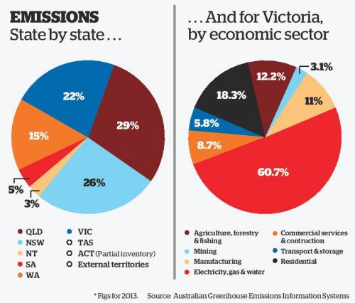
Figure 4.16: Pie charts rely on colour to differentiate categories (Stanton and Alcorn 2016).

Pie charts have spawned many variations. Wired Staff (2008) presented examples of doughnuts charts (pie charts with a hole in the middle) to visualise the changing caloric composition of diets across select countries (see Figure 4.17). The size of the doughnuts represents calories and each segment of the doughnuts represent the proportion of calories that come from major food groups. Each row represents a different three year interval, starting in 1969-1971 and comparing it to 2001-2003. Both size and the area of each segment are difficult to visually compare across countries and time. For example, is the proportional composition of sugar and sweeteners different across time for Brazil? It is very hard to tell with a reasonable degree of accuracy. While eye-catching, the visuals miss the mark.

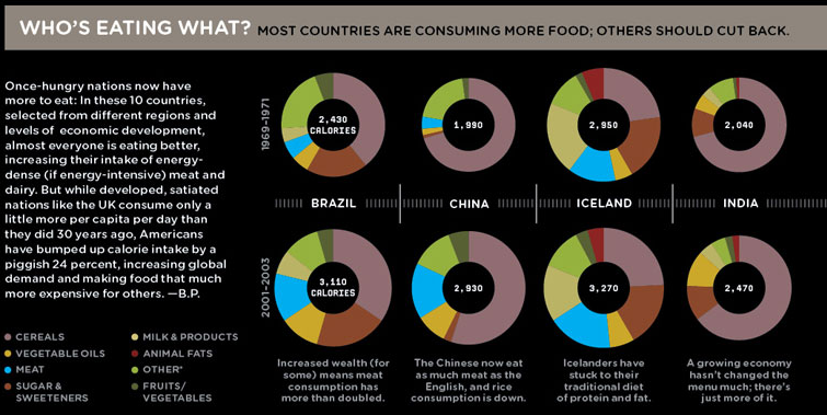
Figure 4.17: Doughnut charts are a variation of the pie chart (Wired Staff 2008).

Figure 4.18 shows another example from The Economist (The Economist Online 2011) comparing different countries on the proportion of time spent on major activity categories for 15-64 year olds. The visuals are mostly unhelpful. The audience if forced to read and compare the numeric values.

Figure 4.18: When visuals fail, the viewers are forced to read the values (The Economist Online 2011).

Are doughnut or pie charts better? Skau and Kosara (2016) found that pie and doughnuts charts are similar in terms of speed and accuracy. If pie and doughnuts charts were not enough, what about pill charts? Daly (2016) used 3D pie charts to show the proportion of drug related convictions in the UK by race (see Figure 4.19). Don’t be fooled. There is only one pie chart. It is just copied to appear like pills. Thankfully, I don’t think pill charts have, or ever will, catch on.

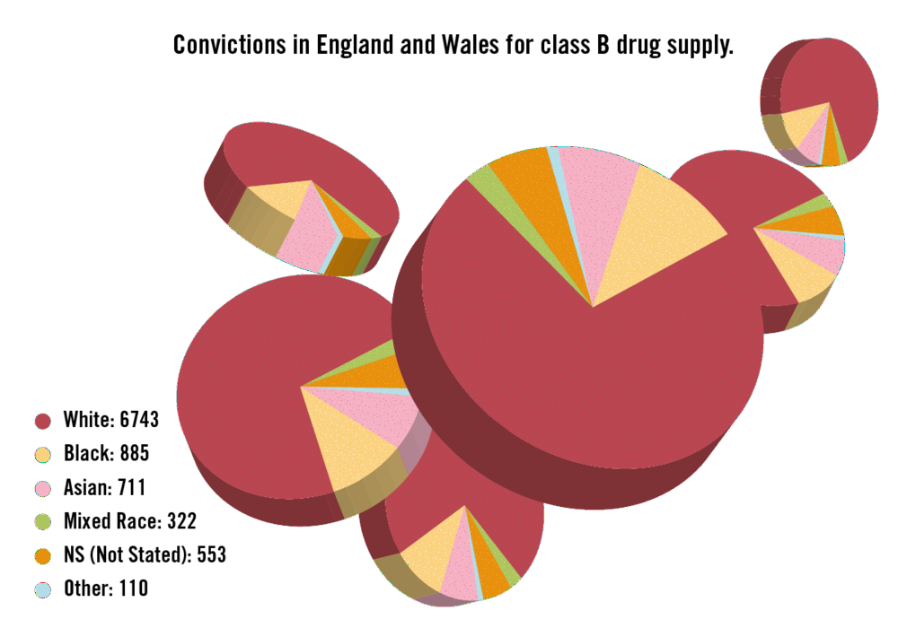
Figure 4.19: Are pill charts the next big thing in data visualisation? (Daly 2016).

So, what’s the issue? Pie charts are cool, right? No, and for very good reason. While pie chart apologists will claim that no other plot can show “parts of a whole” as well as a pie chart, we have already hinted at the main issue. Angle and area have low accuracy for representing numeric values as pointed out by Cleveland and McGill (1985). This makes the proportions represented in the pie chart a lot harder to judge compared to position on an x or y axis. The problem is very pronounced when the proportions are similar. Consider Figure 4.20.

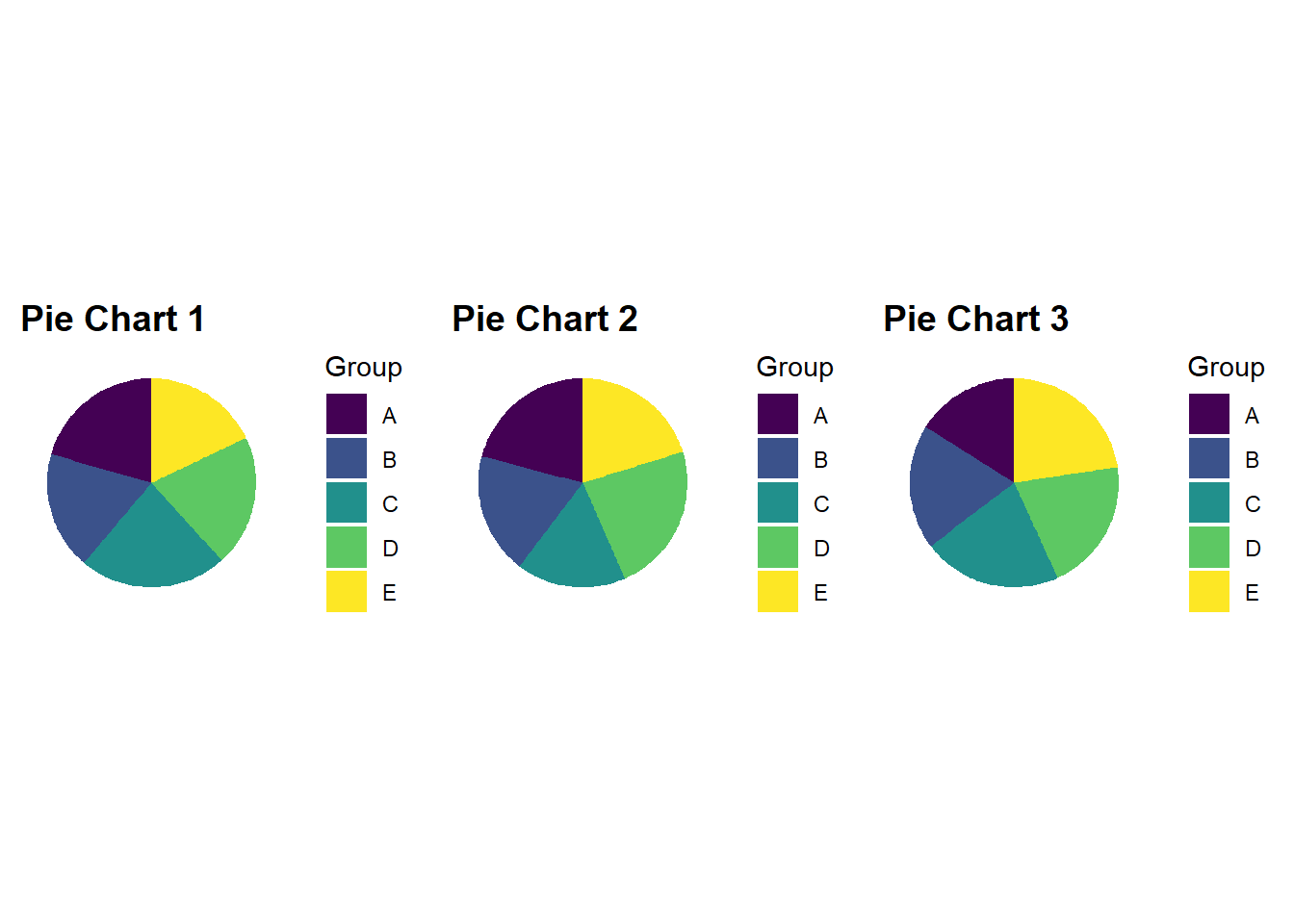
Figure 4.20: When values in a pie chart are similar, fast, accurate comparisons become difficult.

You might be surprised to know that there is quite a bit of difference between some of the proportions in each pie chart. This is made painfully obvious in the bar charts below.

Figure 4.21

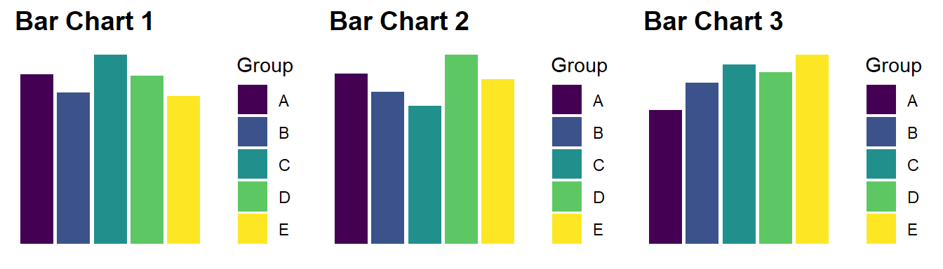
Figure 4.21: Bar charts are always more accurate than pie charts.

Empirical research hasn’t identified a clear winner. For example, Croxton and Stryker (1927) (Yes, pie charts have been controversial for a long time!) found evidence that pie and bar chart accuracy depends on the specific proportions being represented. This suggests that the accuracy of bar vs. pie depends on the data. Regardless of accuracy, there are still other reasons that pie charts are problematic. Here is list of the issues discussed so far as well as the other known issues:

• Area and angle lack visual accuracy compared to position (e.g. bar charts)
• Pie charts perform poorly when proportions are similar
• Pie charts rely on colour to differentiate between segments. Therefore, colour needs to be used with caution.
• Pie charts are limited in the number of categories they can present effectively.
• Pie charts with very small proportions are hard to see and label.

Why are pie charts, and its variations, ubiquitous despite these concerns (Spence 2005)? Gelman and Unwin (2013) differentiates between statistical data graphics and infographics, where the later focuses on grabbing attention and the former on facilitating understanding about patterns present in the data. For Gelman and Unwin (2013) pie charts are considered an info graph because they appear to readily grab peoples’ attention. Cawthon (2007) suggests that this may be explained by their findings which showed that people prefer the aesthetics of visualisations that exhibit organic qualities (smooth, continuous and natural forms) as opposed to the artificial qualities of straight lines, angles and equal spacing. Form and function are in constant tension in data visualisation. Balance is the key.

Simon Weller, a former student from the course that inspired this textbook, shows how the The Economist’s (The Economist Online 2011) doughnut chart can be visualised effectively using the “humble” bar chart (see Figure 4.18). While it might not be as visually striking at the original, function is restored. The audience can rapidly compare countries on where they are spending more or less time. A feat that could only be achieved in the original by reading the value labels.

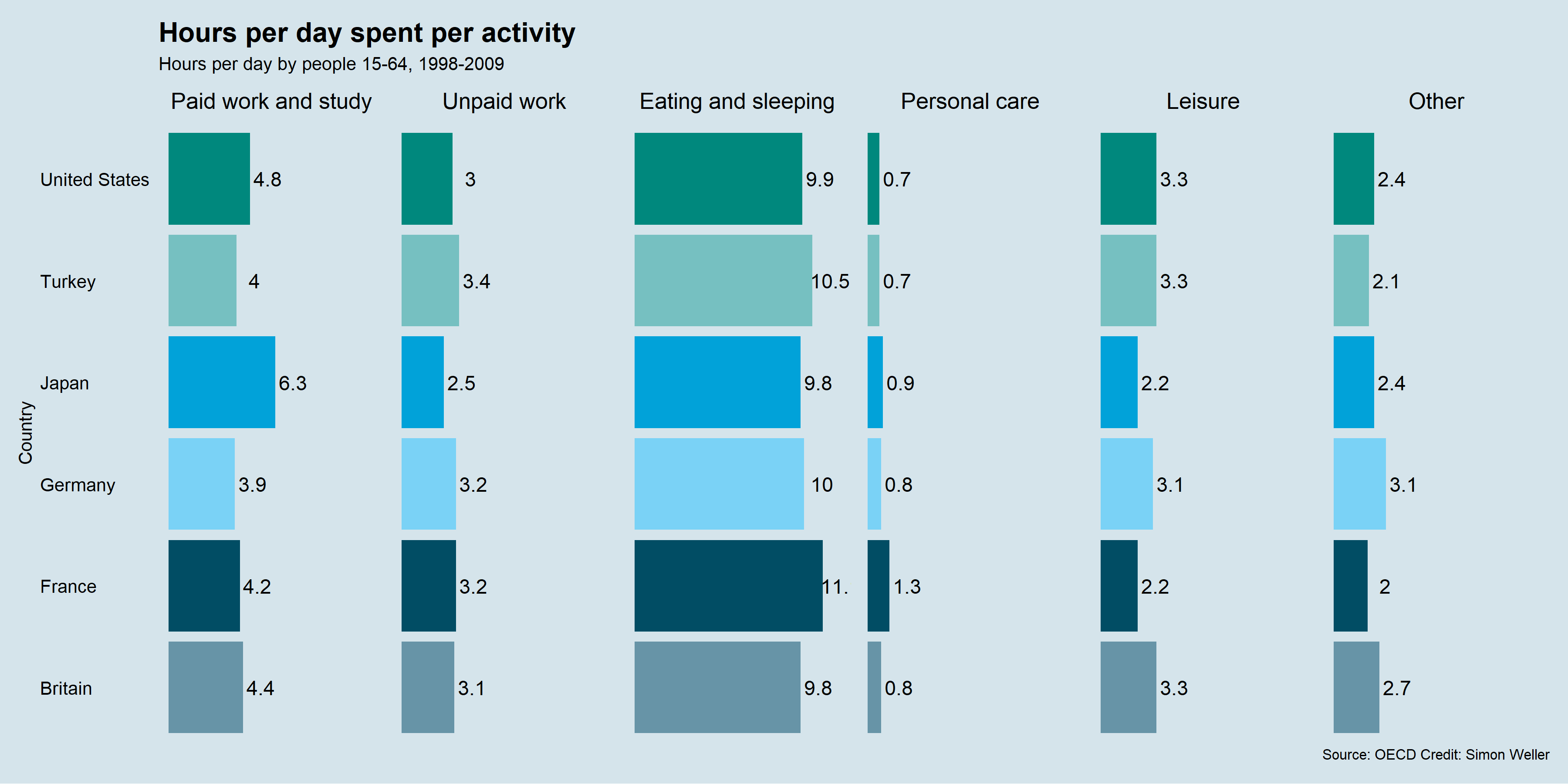
Figure 4.22: Simon Weller, a former student, fixed The Economist Online (2011)’s doughnut charts using faceted bar charts.

So, what is the take home message? Pies and doughnuts are for eating. Don’t be tempted to use them in data visualisation. Especially when the humble bar chart works very well. Figure 4.23 shows a nice gif from Joey Cherdarchuk (2014) from Darkhorse Analytics that captures the lesson well (only available online).

Figure 4.23: Devour the pie! (Cherdarchuk 2014).

4.3.2 Truncated Axis

When we have a count or ratio variable, truncating an axis, or shortening it, will distort the relative differences between groups (Pandey et al. 2015). This is commonly seen in bar charts such as Leo (2019) from The Economist (see Figure 4.24). In Leo (2019)’s exposé of bad data visualisations from The Economist, you can see the impact of truncating the axis in the original bar chart of Jeremy Corbyn’s likes per post on Facebook. The second bar chart removes the truncated axis which corrects the proportionality to other accounts. The second, more accurate, bar chart shows just how much more popular Jeremy’s posts are to other accounts.

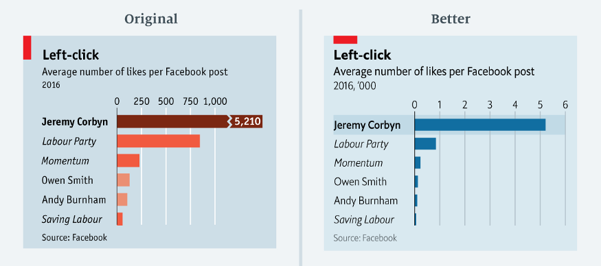
Figure 4.24: A truncated axis can severely distort a data visualisation (Leo 2019).

Here is another example of a strange truncated axis reported by Stafford and White (2018) from Car and Driver (see Figure 4.25). It is not clear from the plot where the x-axis starts. The assumption would be 0. This means the first half of the x-axis is equal to 30 miles per gallon (MPG), and the second half of the axis 100 MPG. Weird indeed.

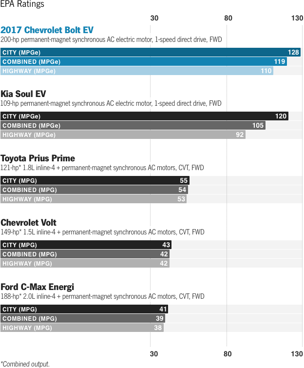
Figure 4.25: An unusual x-axis (Stafford and White 2018).

To see what effect this has on the visualisation, let’s do a simple bar chart for comparison. As you can see in Figure 4.26, the original visualisation underestimates the MPG difference of the Chevrolet Bolt and Kia Soul relative to the other cars.

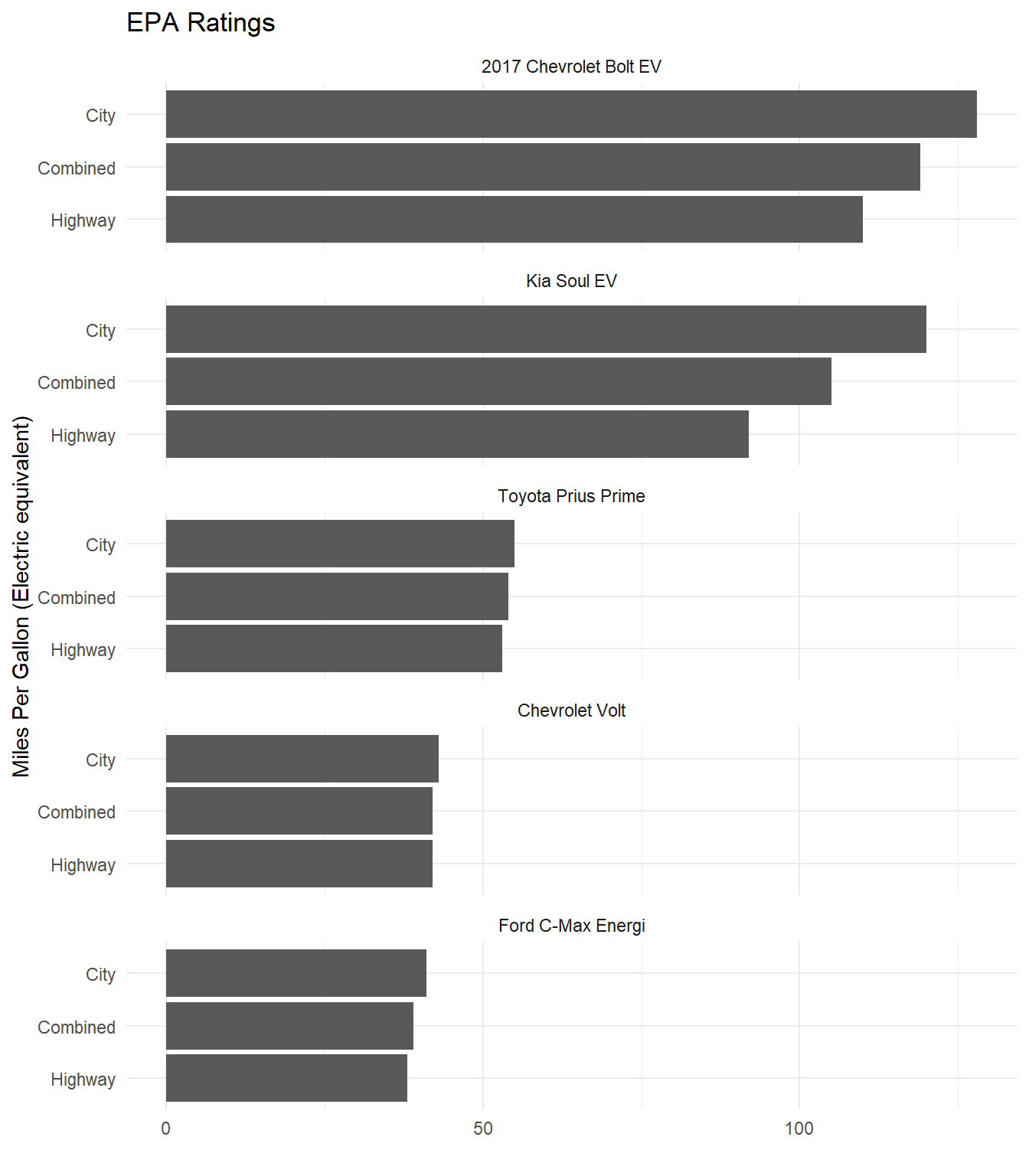
Figure 4.26: Fixing the unusual x-axis in Stafford and White (2018).

Parkinson (2013) presents a more typical example where the y-axis does not start at 0 (see Figure 4.27). This means our sense of the relative difference in British men’s average height at age 21 across time is grossly exaggerated.

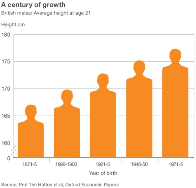
Figure 4.27: Notice the truncated y-axis (Parkinson 2013).

Look at Figure 4.28 which does not truncate the y-axis. Now this presents a very different picture and puts the height increase in perspective. Taller, yes, but not by the magnitude visually depicted in Parkinson (2013). Parkinson (2013) does include a visual cue to alert the reader to the truncated axis. You will notice two small slashes that break the axis. However, this visual cue is not strong enough and many readers will miss it.

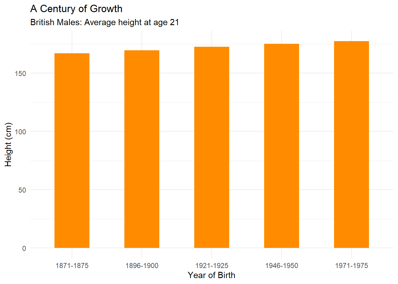
Figure 4.28: Fixing the y-axis of Parkinson (2013).

4.3.3 Area and Size as Quantity

Cleveland and McGill (1985) have already shown that area and size rank lower than position in terms of accuracy when visualising a quantitative variable. Pie charts are one example of this issue. However, the way in which area and size are scaled can also be problematic. Take the bar chart from ACMA Research and Analysis Section (2015) for example (see Figure 4.29). It is not clear what the y-axis represents. Is it the number of mobile-only phone users or the percentage of the Australian population who are mobile-only phone users? Both are reported, but they are not the same thing. As the population size grows each year, looking at the total number of users can be misleading. The percentages are more useful. The bars also have a width value which creates an area/size for each bar depicted as a mobile phone. It appears the aspect ratio of each bar is fixed, so the “bars” appear like an iPhone. There is little information provided that explains how the area or size of each phone was scaled.

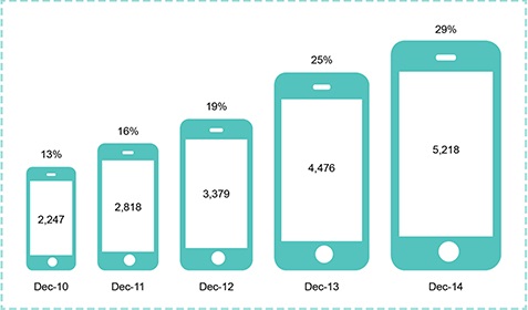
Figure 4.29: Growth of the mobile-only phone user, December 2010 to December 2014 (ACMA Research and Analysis Section 2015).

Let’s figure out if this unusual bar chart has deceived us. First, let’s do some image manipulation. If you take 13% and double it, you get 26%. Therefore, the Dec-13 area should be about twice the area of Dec-10. According to Figure 4.30, it is not. Dec-13 appears close to four times larger. This suggests that the size of each phone might be scaled as Area = Length * Width.

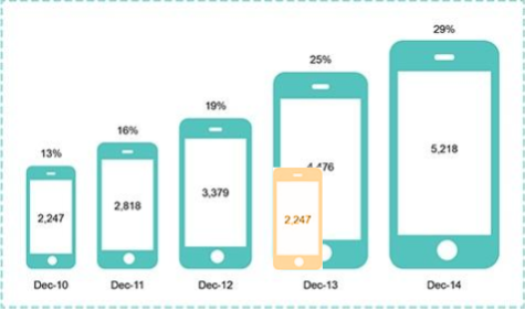
Figure 4.30: Area is not scaled correctly (ACMA Research and Analysis Section 2015).

Figure 4.31 shows the issue that this presents. Area and size needs to be treated carefully as it can easily deceive (Pandey et al. 2015). Pandey et al. (2015) state that best practice with area is using a 1:1 mapping between a quantitative variable and the area depicted visually. We checked this by superimposing the phones from Dec-10 and Dec-13 and found the mapping to be approximately 1:4.

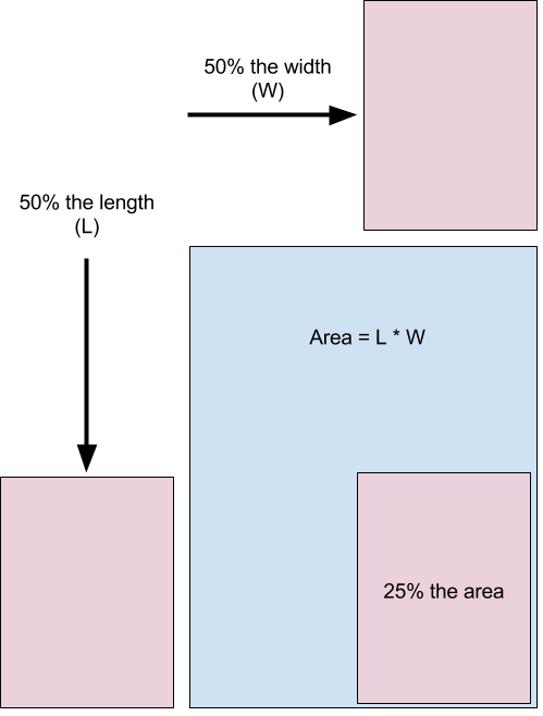
Figure 4.31: When using area, use a 1:1 mapping to avoid distortion (Pandey et al. 2015).

How do you fix this? The best option is to use position on a y-axis. This is time series data, so you should use a connected line graph. The result is clearer and more accurate (see Figure 4.32).

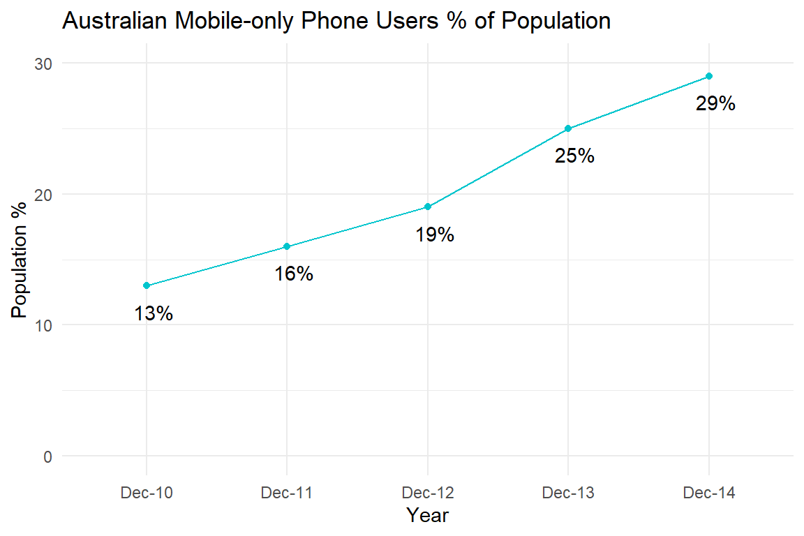
Figure 4.32: Fixing the mobile phone bar chart using a time-series plot.

How would a 1:1 mapping appear if we stuck to size? This is shown in Figure 4.33. The areas are now accurate, but the connected line plot’s use of position on the y-axis is far more accurate. Using this corrected size chart, look back to 4.29 which drastically exaggerates the change across time.

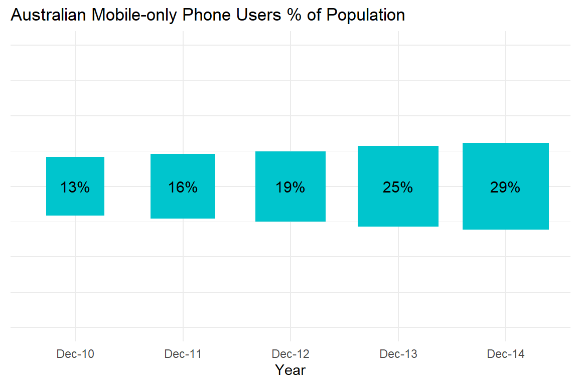
Figure 4.33: 1:1 size mapping for the mobile phone bar chart.

4.3.4 Aspect Ratio

Changing the aspect ratio of a plot can also deceive (Pandey et al. 2015). The aspect ratio refers to the ratio of a plot’s width:height. This is explained in Figure 4.34.

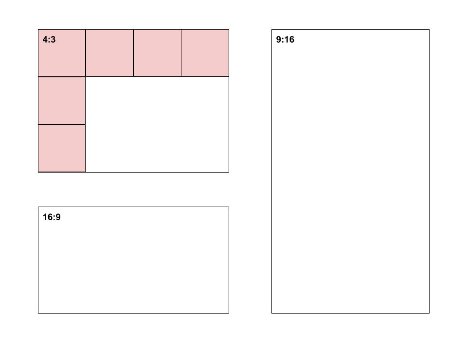
Figure 4.34: Aspect ratio explained.

Plots that rely on showing a change across time, such as a time-series plots, are sensitive to this issue because the aspect ratio directly impacts the perceived rate of change. Let’s take a look at how easy it is to manipulate. The time series plot of Average temperative anomaly, Global by Ritchie and Roser (2017) from Our World in Data will be used as an example (see Figure 4.35).

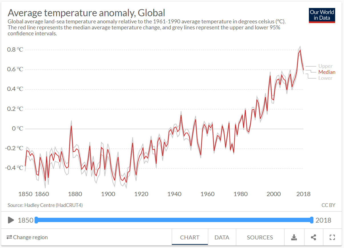
Figure 4.35: Average temperature anomaly time series plot by Ritchie and Roser (2017).

The original is reproduced closely in Figure 4.36. We will use this to manipulate the aspect ratio.

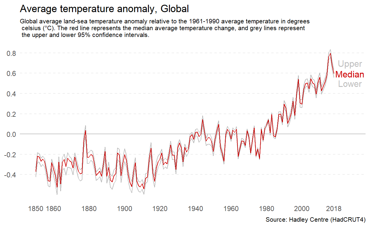
Figure 4.36: A reproduction of the temperature anomaly time series plot by Ritchie and Roser (2017).

If you want to minimise the perceived change, you can increase the width of the plot relative to the height. Figure 4.37 has an aspect ratio of 3:1. This makes the rate of change across time appear more gradual.

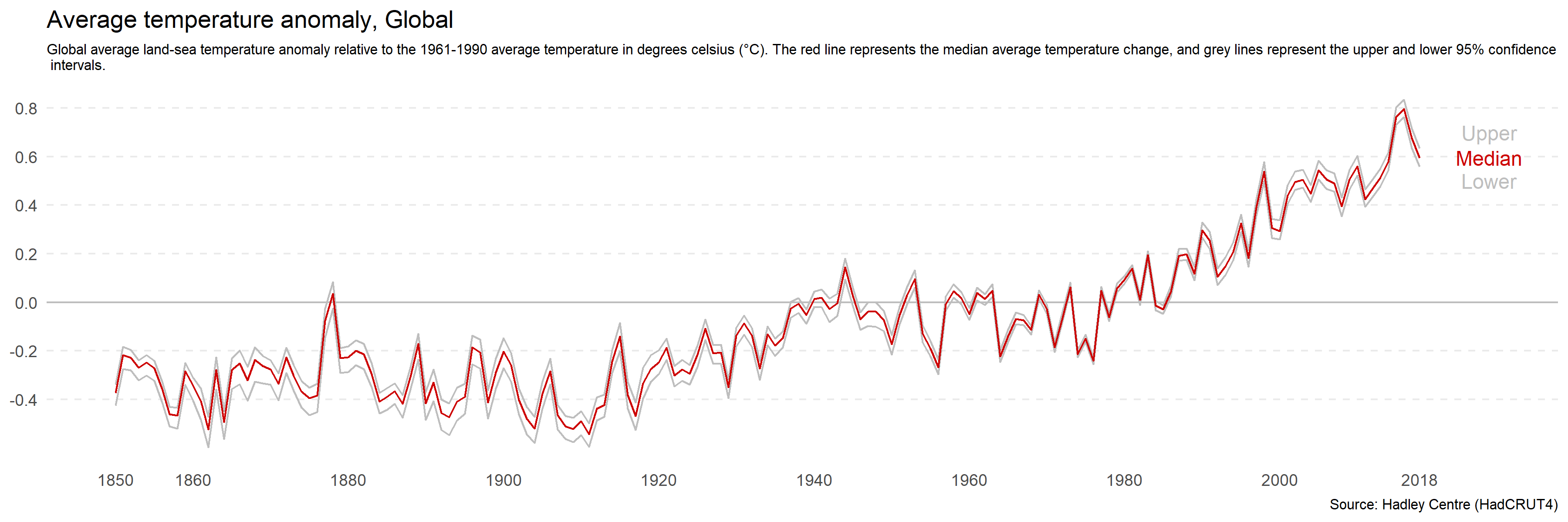
Figure 4.37: Increasing the width of a plot relative to height minimise perceived differences.

You can do the opposite to make the rate of change appear more rapid by increasing the height of the plot relative to the width. Figure 4.38 has an aspect ratio of 3:5. The change appears sudden and drastic.

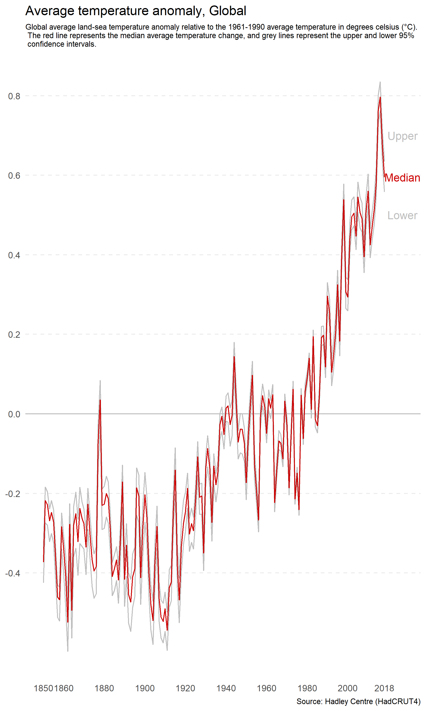
Figure 4.38: Increasing the height of a plot relative to width increases perceived differences.

Beware of this distortion when setting the size of your plots. You do not want to unwittingly mislead your audience. There is no magic ratio. Use common sense and avoid extreme ratios. This issue is more relevant than ever with the widespread use of responsive web design, which means that websites and web-based data visualisations are capable of re-scaling based on screen size and viewing device. This means it is important to check the appearance of your plots on different devices and fix the aspect ratio if distortions are likely to occur.

4.3.5 Ignoring Convention

There are many conventions in data visualisation. For example, the horizontal axis is referred to as x. Time is presented as progressing from left to right and growth moving from the bottom of plot to the top. There are historical, cultural and educational reasons underlying these conventions. Convention is important because it allows you to make assumptions about your audience. The audiences’ prior experiences and expectations determine much about how they will perceive a data visualisation.

When you ignore these conventions, you risk misleading or confusing your audience. For example, Chan (2014), as cited in Engel (2014), presents a time series plot of gun-related deaths in Florida before and after the enactment of the “Stand Your Ground” law in 2005 (see Figure 4.39). This law made it legal to use deadly force for self-defense or the self-defense of others. If you take a quick glance at the plot, you would be forgiven for thinking that the act corresponded to a drastic decrease in gun-related deaths. However, you would be wrong. Notice the inversion of the y-axis.

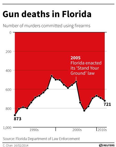
Figure 4.39: The infamous Gun Deaths in Florida plot by Chan (2014) as cited in Engel (2014).

Flipping the plot upside down fixes the problem (see Figure 4.40).

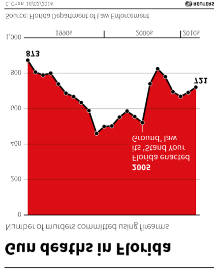
Figure 4.40: Inverting the Gun Deaths in Florida plot by Chan (2014) as cited in Engel (2014).

This visualisation drew a lot of criticism for being deceptive. However, not everyone agreed. For example, Kirk (2014) argued it was not deceptive and depended on how it was interpreted. Kirk (2014) reasoned that the area coloured red was what visually corresponded to total deaths. The original designer, Christine Chan, explained that they drew inspiration from a similar visualisation named Iraq’s bloody toll by Scarr (2011) (see Figure 4.41). Red is associated with blood and violence, and inverting the axis made it appear like dripping blood. Regardless, ignoring conventions can be used to deceive, confuse and ignite the internet against you. Stick to conventions.

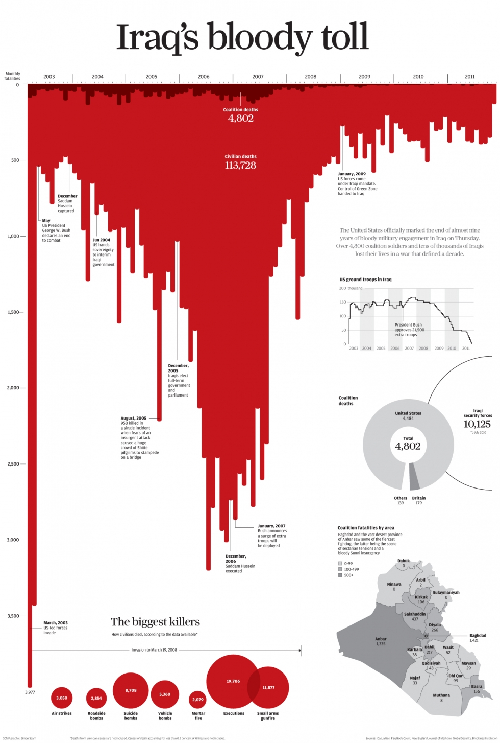
Figure 4.41: Iraq’s bloody toll by Scarr (2011).

4.3.6 Dual Axes

The use of dual axes in data visualisation isn’t uncommon. This means that instead of one variable being positioned on the y-axis, two variables are plotted instead, one on the left and one on the right. Look Figure 4.42 from The Economist (2016) showing how the weight and neck size of dogs in the UK have shrunk overtime in what appears to be a perfect relationship.

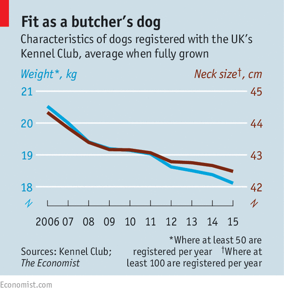
Figure 4.42: Dual axes in The Ecconomist (The Economist 2016).

However, Leo (2019) was critical of this orginal plot:

In the original chart, both scales decrease by three units (from 21 to 18 on the left; from 45 to 42 on the right). In percentage terms, the left scale decreases by 14% while the right goes down by 7%.”

In, other words, while both neck and weight go down, weight has decreased quicker than neck size. Leo corrects this visualisation by adjusting the scales so that each year shows a proportional change (see Figure 4.43).

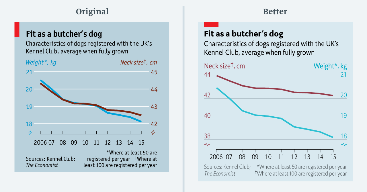
Figure 4.43: Improving a dual axes plot (Leo 2019).

In general, dual axis plots should be avoided because they are easy to manipulate and, even when done well, are prone to misinterpretation. The secondary scale can often go unnoticed and are generally difficult to understand. Just how easy are they to manipulate? Let’s take a look. Figure 4.44 was adapted from Reddit user Buckbuckyyy (2019). The data were taken from the City of New York website (NYC OpenData 2019). The plot shows that despite the NYC population increasing, water use has declined.

Figure 4.44: NYC Water Consumption and Population 1979 - 2017.

The important thing to keep in mind when thinking about dual axes is that the scaling of the secondary axis is completely arbitrary and has to be carefully set by the designer so that the superimposition of the two variables is accurately presented. This is difficult to get right and prone to deception. Figure 4.45 presents an alternative scaling. It appears water consumption has plummeted.

Figure 4.45: It is easy to manipulate a dual axes plot by manipulating the scale. Water use has plummeted!

It is not hard to show something different. For example, that the population has exploded (see Figure 4.46). While extreme, you get the point.

Figure 4.46: Population has exploded!

User experiments by Isenberg et al. (2011) have shed light on the issues of interpreting dual axis plots. Isenberg et al. (2011) used superimposed charts for dual “scale” plots. The second axis was used to “focus” or “zoom” in on a specific region of a plot to facilitate comparisons to other regions. While not directly related to the use of dual “axis” plots for the purpose of visualising two variables on the same axis, the findings of the paper are still relevant. Participants from the study reported that the superimposed charts were the most confusing and time consuming to interpret. They were also the least accurate in terms of other methods tested in the experiment. What other methods are appropriate? Few (2008), Evergreen (2020) and Rost (2018), recommend aligning multiple plots (side-by-side or bottom and top) as they are easier to implement and easy to understand (see Figure 4.47).

Figure 4.47: Aligning individual plots is a preferred alternative to dual axes plots (Few 2008; Evergreen 2020; Rost 2018).

Another approach suggested by Few (2008) and Rost (2018) would be to plot indexed values. For example, convert each variable to a percentage change based on a reference year. This standardises the two variables to a common scale. However, there are issues if the magnitude of the change is drastically different between the variables. Converting two variables into a single ratio variable is also sometimes possible. For example, you can use the ratio for water use per person per day (see Figure 4.48).

Figure 4.48: A ratio of two quantitative variables avoids dual axes.

Connected line plots might also be a useful alternative as demonstrated in Figure 4.49, although they are likely to be unfamiliar and time-consuming for the audience (Rost 2018; Evergreen 2020).

Figure 4.49: Connecting points by time allows the viewer to correlate two time-based variables.

As a general rule, avoid using dual axis plots. There are too many issues to confidently deal with and better alternatives are available.

4.3.7 Other Poor Scaling Methods

You have already considered a number of deceptive methods related to poor scaling - truncated axes, inverted axes and dual axes. Let’s consider a few more. Cleverland, Diaconis, and McGill (1982) conducted a seminal experiment where they manipulated the scale of a scatter plot in order to determine its effect on judgement of correlation. In one scatter plot, the scale was set to the range of the bivariate data (see plot A in Figure 4.50) and in the second, the scale on both the x and y axis were increased (see plot B in Figure 4.50). This had the effect of “zooming out” on the data. The data are the same in both Plot A and B and the correlation is \(r=\) 0.89.

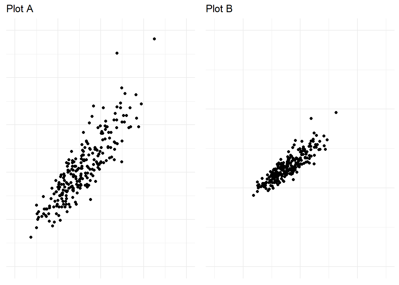
Figure 4.50: Zooming out in a scatter plot can exaggerate trends.

When asked to judge the correlation of the bivariate data across 19 different scatter plots where the scale and correlation were manipulated. Participants were found to rate the correlation in the plots with an increased scale (Plot B above) significantly higher than plots with a smaller scale. This was the first experiment to show empirically how the scale of a plot impacts interpretation.

Yanofsky (2015) explains poor scaling on the y-axis in time-series plots can render them useless. For example, truncating the axis in bar charts that aim to facilitate proportional comparison across categories is considered bad practice. However, this rule does not apply well to many time-series plots. Take Yanofsky (2015)’s example of US Gross Domestic Product (GDP) over time shown in Figure 4.51. Including 0 in the plot hides the impact of the Global Financial Crisis (GFC) due to the scale of GDP being in the trillions.

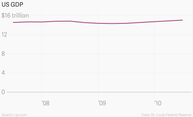
Figure 4.51: US GDP across time by Yanofsky (2015). Because the y-axis scale starts at 0, the time series trend is barely noticeable.

Plotting the data starting at 14 billion on the y-axis solves this issue and allows the reader to see the clear slump characterised by the GFC (see Figure 4.52).

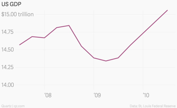
Figure 4.52: Scaling the y-axis to start at 14bn ensures the sump of Global Financial Crisis can be seen (Yanofsky 2015).

When manipulating the scale of your data visualisation keep examples like these in mind. Poor scaling can easily exaggerate or understate trends in the data. Scale your visualisations accurately and in a way that communicates the right message.

4.3.8 Visual Bombardment

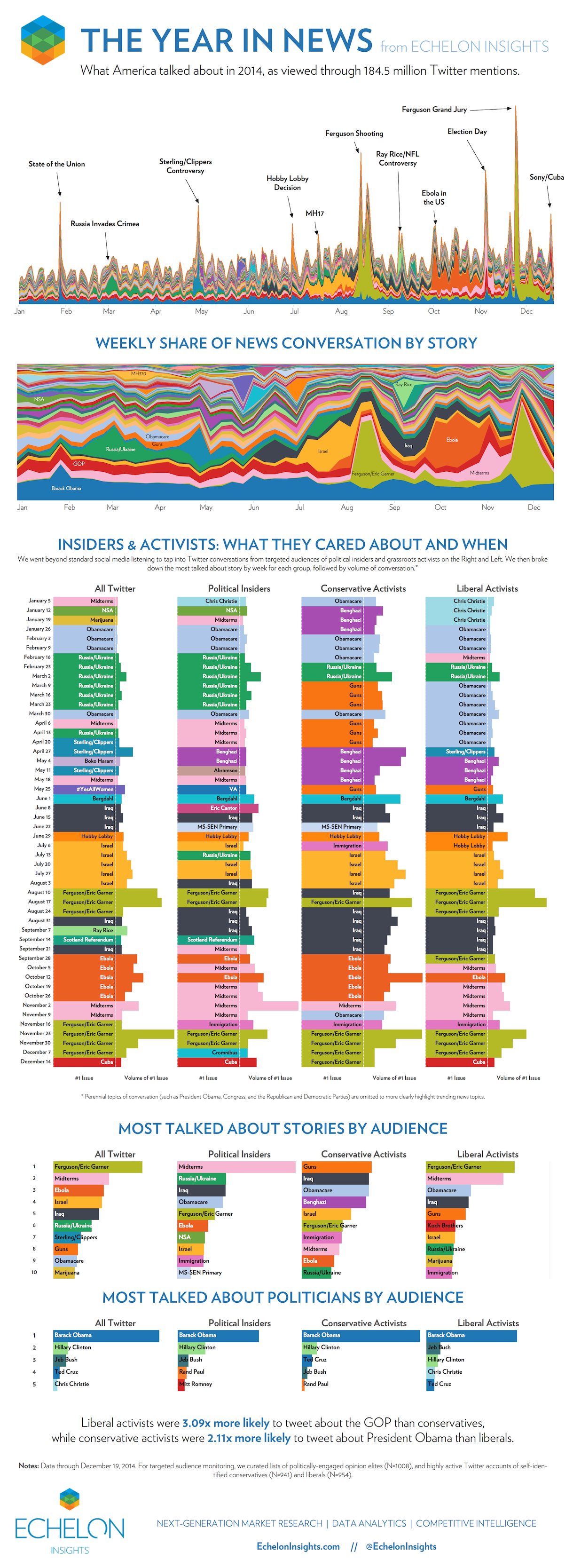
If you want to say anything about your data, make a data visualisation that overwhelms your audience and distracts them from the real message in the data. Use heaps of colour, groups, data etc. to paint a really complex visual message. You want your audience to give up making any sense of the visuals and then rely on text/narration/video to tell them the story or leave them completely confused. Echelon Insights (2014) provide a great example in Figure 4.53. Echelon Insights visualised 184.5 million 2014 Twitter mentions of news stories and presented the following stacked and filled time series plots.

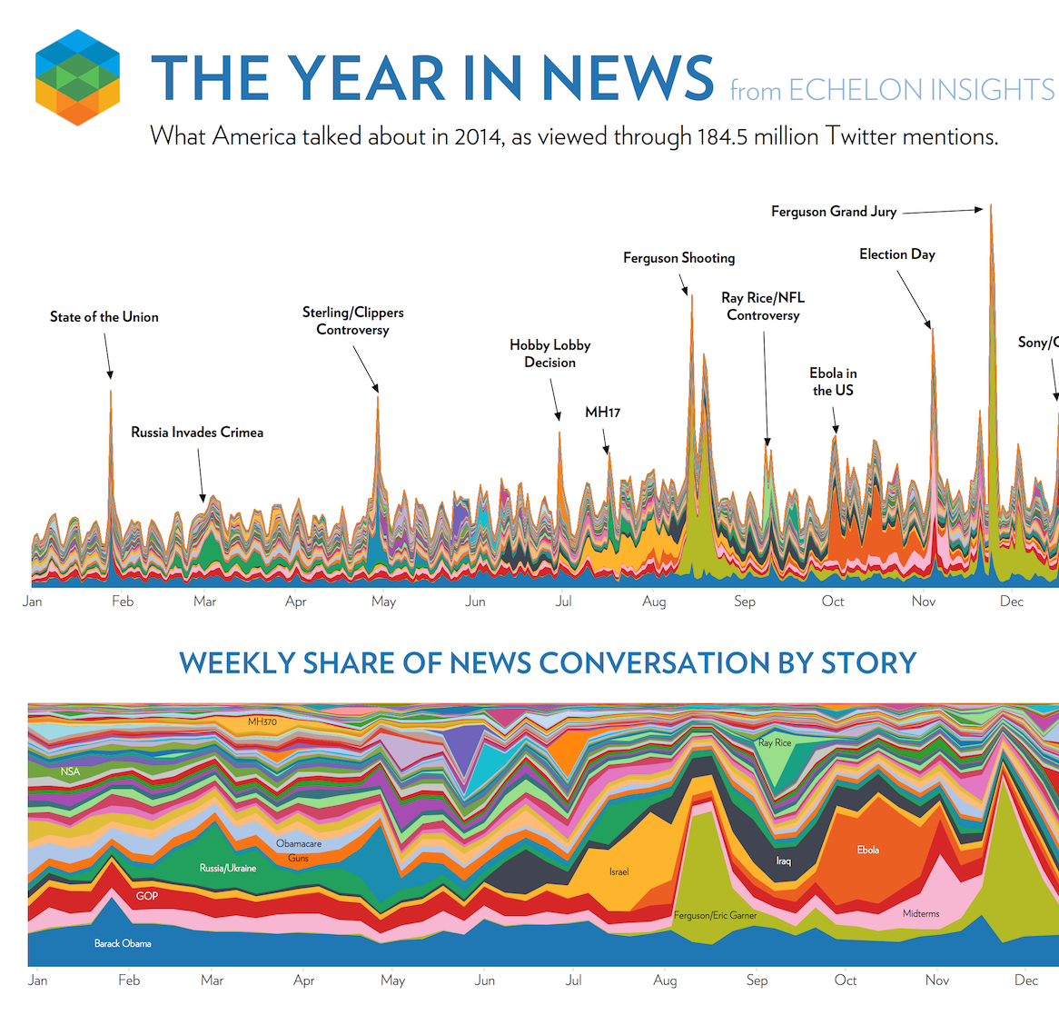
Figure 4.53: Visual bombardment confuses your audience (Echelon Insights 2014).

Many people would look at these visualisations and be impressed. 184.5 million Tweets! Yah, data science! Echelon Insights are overwhelming their audience to flex their big data muscle. Once you see past that, the visuals are lacking. You simply cannot see, nor do you need to see so many news topics depicted by countless colours. The annotations corresponding to spikes in the Twittersphere are the only redeeming feature. Visual bombardment is a common side-effect of big data.

Let’s take a look at another example. A Bird’s Eye View of Pharmaceutical Research and Development by Aero Data Lab (2019) exhibits an impressive range of strategies to bombard the audience (see Figure 4.54, the full screen version is available here). Despite good intentions, the plot is largely incomprehensible. There are far too many disease/conditions (800) that require the viewer to scroll down and lose sight of other diseases (click on the image below to see the full visualisation), inclusion of several variables (y = disease, x = time, colour = company, size = number of clinical trial subjects, shape = status of clinical trial) and extensive overplotting of bubbles.

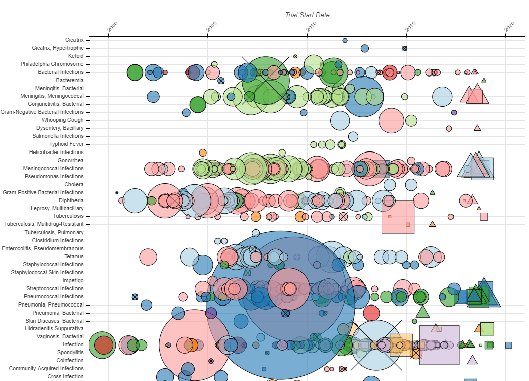
Figure 4.54: To many variables! (Aero Data Lab 2019).

Remember Kirk (2012)’s third guiding principle, Creating accessibility through intuitive design. Data visualisation is based on human visual communication. Whilst the computers you have access to today are more than capable of creating big, complex plots, keep in mind that a human brain will need to interpret it. Respect the cognitive and perceptual limits of your audience. It is your job to make the data visualisation accessible.

4.3.9 Concluding Thoughts

This chapter has taken a close look at some of the common methods used in data visualisation than can potentially deceive your audience. You also considered strategies for avoiding similar deception in your own work. These are some of the most common issues, but, keep in mind, there are many other examples and many yet to be discovered. You must always take reasonable steps to avoid deception. Otherwise you will fail in your obligations to the audience.

References

“2025 Southwest United States Measles Outbreak.” 2026. In Wikipedia. https://en.wikipedia.org/w/index.php?title=2025_Southwest_United_States_measles_outbreak&oldid=1338934452.

ACMA Research and Analysis Section. 2015. “Australians get mobile.” https://www.acma.gov.au/theACMA/engage-blogs/engage-blogs/Research-snapshots/Australians-get-mobile.

Aero Data Lab. 2019. “A bird’s eye view of pharmaceutical research and development.” https://www.aerodatalab.org/birds-eye-view-of-research-landscape.

Australian Bureau of Statistics. 2023. “National Health Survey, 2022.” https://www.abs.gov.au/statistics/health/health-conditions-and-risks/national-health-survey/2022.

Australian Institute of Health and Welfare. 2021. “Eye Health.” https://www.aihw.gov.au/reports/eye-health/eye-health/contents/new.

———. 2024a. “People with Disability in Australia, Prevalence of Disability - Australian Institute of Health and Welfare.” https://www.aihw.gov.au/reports/disability/people-with-disability-in-australia/contents/people-with-disability/prevalence-of-disability.

———. 2024b. “Eye Health Measures for Aboriginal and Torres Strait Islander People 2024.” https://www.aihw.gov.au/reports/indigenous-australians/eye-health-measures-2024/data.

Bresciani, S., and M. J. Eppler. 2008. “The risks of visualization: A classification of disadvantages associated with graphic representations of information.” Institute for Corporate Communication. https://pdfs.semanticscholar.org/23d2/3f5152c9b8b34f104b43d1c862ee62d2edac.pdf.

Brewer, C. A., and M. Harrower. 2019. “ColourBrewer 2.0 web tool.” http://colorbrewer2.org.

Brown, L. M., S. A. Brewster, S. A. Ramloll, R. Burton, and B. Riedel. 2003. “Design Guidelines for Audio Presentation of Graphs and Tables.” In Proceedings of the 9th International Conference on Auditory Display (ICAD), 284–87.

Buckbuckyyy. 2019. “NYC water consumption over the years from 1979-2017.” https://www.reddit.com/r/dataisbeautiful/comments/be6yww/oc{\_}nyc{\_}water{\_}consumption{\_}over{\_}the{\_}years{\_}from/.

Cawthon, Nick. 2007. “Qualities of perceived aesthetic in data visualization.” In Proceedings of the 2007 Conference on Designing for User eXperiences - DUX ’07, 1. New York, New York, USA: ACM Press. https://doi.org/10.1145/1389908.1389920.

Center for Accessibility Australia. 2024. “Understanding Accessibility.” https://www.accessibility.org.au/guides/.

Cherdarchuk, Joey. 2014. “Salvaging the pie.” https://www.darkhorseanalytics.com/blog/salvaging-the-pie.

Chun, Russell. 2017. “Redundant Encoding in Data Visualizations: Assessing Perceptual Accuracy and Speed.” Visual Communication Quarterly 24 (July): 135–48. https://doi.org/10.1080/15551393.2017.1343153.

Cleveland, W. S. 1994. The Elements of Graphing Data. Revised Edition. Hobart Press.

Cleveland, W. S., and R. McGill. 1985. “Graphical perception and graphical methods for analyzing scientific data.” Science 229 (4716): 828–33.

Cleverland, W. S., P. Diaconis, and R. McGill. 1982. “Variables on scatterplots look more highly correlated when the scales are increased.” Science 216 (4550): 1138–41. https://doi.org/10.1126/science.216.4550.1138.

Cowan, Nelson. 2010. “The Magical Mystery Four: How Is Working Memory Capacity Limited, and Why?” Current Directions in Psychological Science 19 (February): 51–57. https://doi.org/10.1177/0963721409359277.

Croxton, Frederick E., and Roy E. Stryker. 1927. “Bar charts versus circle diagrams.” Journal of the American Statistical Association 22 (160): 473. https://doi.org/10.2307/2276829.

Daly, Max. 2016. “Exclusive: New conviction data tells us how the UK sells drugs.” https://www.vice.com/en{\_}us/article/dp5npk/foi-uk-drug-conviction-ethnicity-282.

Dattani, S., and F. Spooner. 2025. “Measles Vaccines Save Millions of Lives Each Year.” Our World in Data, May. https://ourworldindata.org/measles-vaccines-save-lives.

Digital NSW. 2023. “A Guide to Digital Accessibility for Colour Blind User.” https://www.digital.nsw.gov.au/article/a-guide-to-digital-accessibility-for-colour-blind-users.

Echelon Insights. 2014. “The year in news.” http://echeloninsights.com/wp-content/uploads/2014/12/theyearinnews20141.png.

Elavsky, F. 2023. “Introduction to Accessible Contrast and Color for Data Visualization.” Observable. https://observablehq.com/@frankelavsky/chartability-contrast-series.

———. 2025. “GitHub - Chartability/POUR-CAF: Chartability, an Inclusive Data Experience Toolkit.” https://github.com/Chartability/POUR-CAF.

———. n.d. “The Chartability Workbook.” https://chartability.github.io/POUR-CAF/.

Elavsky, F., Cynthia Bennett, and Dominik Moritz. 2022. “How Accessible Is My Visualization? Evaluating Visualization Accessibility with Chartability.” Computer Graphics Forum 41 (June): 57–70. https://doi.org/10.1111/cgf.14522.

Energy Rating. 2019. “Water heating.” http://www.energyrating.gov.au/products/water-heaters.

Engel, P. 2014. “This chart shows what happened to gun deaths in Florida after ’Stand Your Ground’ was enacted.” https://www.businessinsider.com.au/gun-deaths-in-florida-increased-with-stand-your-ground-2014.

Evergreen, S. 2020. “Two alternatives to using a second y-axis.” http://stephanieevergreen.com/two-alternatives-to-using-a-second-y-axis/.

Evergreen, S., and A. K. Emery. 2016. “Updated data visualization checklist.” https://stephanieevergreen.com/updated-data-visualization-checklist/.

Evershed, N. 2024. “Noisycharts-Npm.” https://github.com/nickjevershed/noisycharts-npm.

Fan, Danyang, Alexa Fay Siu, Hrishikesh Rao, Gene Sung Ho Kim, Xavier Vazquez, Lucy Greco, Sile O’modhrain, and Sean Follmer. 2023. “The Accessibility of Data Visualizations on the Web for Screen Reader Users: Practices and Experiences During COVID-19.” ACM Transactions on Accessible Computing 16 (March). https://doi.org/10.1145/3557899.

Few, S. 2008. “Dual-scaled axes in graphs. Are they ever the best solution?” https://www.perceptualedge.com/articles/visual{\_}business{\_}intelligence/dual-scaled{\_}axes.pdf.

Flowers, J. H. 2005. “Thirteen Years of Reflection on Auditory Graphing: Promises, Pitfalls, and Potential New Directions.” In Proceedings of ICAD 05-Eleventh Meeting of the International Conference on Auditory Display, 406–9.

Ganner, J., A. Mrva-Montoya, M. Park, and K. Duncan. 2023. Books Without Barriers: A Practical Guide to Inclusive Publishing. Institute of Professional Editors; Australian Publishers Association. https://publishers.asn.au/BooksWithoutBarriers.

Garnier, S., N. Ross, B. Rudis, M. Sciaini, A. P. Camargo, and C. Scherer. 2024. “Viridis(lite) - Colorblind-Friendly Color Maps for r.” Zenodo. https://doi.org/10.5281/zenodo.4679423.

Gelman, Andrew, and Antony Unwin. 2013. “Infovis and statistical graphics: Different goals, different looks.” Journal of Computational and Graphical Statistics 22 (1): 2–28. https://doi.org/10.1080/10618600.2012.761137.

Isenberg, P., A. Bezerianos, Pierre Dragicevic, and Jean-Daniel Fekete. 2011. “A study on dual-scale data charts.” IEEE Transactions on Visualization and Computer Graphics 17 (12): 2469–78. https://doi.org/10.1109/TVCG.2011.160.

Jin, Tao, Chunpeng Chen, Yuting Xia, Xinyu Liu, and Xiaoxu Liu. 2025. “Do Redundant Graphical Attributes Reduce Decision-Making Efficiency?” Ergonomics 68 (February): 213–22. https://doi.org/10.1080/00140139.2024.2316314.

Kirk, A. 2012. Data visualization: a successful design process. Birmingham, UK: Packt Publishing Ltd.

———. 2014. “The fine line between confusion and deception.” https://www.visualisingdata.com/2014/04/the-fine-line-between-confusion-and-deception/.

Kroes, E. 2021. “Color and Contrast, What Does It Mean?” ErikKroes.nl. https://www.erikkroes.nl/blog/color-and-contrast/.

Leo, S. 2019. “Mistakes, we’ve drawn a few.” https://medium.economist.com/mistakes-weve-drawn-a-few-8cdd8a42d368.

MacDonald, L. W. 1999. “Using color effectively in computer graphics.” IEEE Computer Graphics and Applications 19 (4): 20–35. https://doi.org/10.1109/38.773961.

Nees, M. A., and B. N. Walker. 2007. “Listener, Task, and Auditory Graph: Toward a Conceptual Model of Auditory Graph Comprehension.” In Proceedings of the 13th International Conference on Auditory Display (ICAD2007), 266–73.

NYC OpenData. 2019. “Water consumption in the New York City.” https://data.cityofnewyork.us/Environment/Water-Consumption-In-The-New-York-City/ia2d-e54m.

Okabe, M., and K. Ito. 2008. “Color Universal Design (CUD): How to Make Figures and Presentations That Are Friendly to Colorblind People.” https://jfly.uni-koeln.de/color/#pallet.

Pandey, Anshul Vikram, Katharina Rall, Margaret L. Satterthwaite, Oded Nov, and Enrico Bertini. 2015. “How deceptive are deceptive visualizations?” In Proceedings of the 33rd Annual ACM Conference on Human Factors in Computing Systems - CHI ’15, 1469–78. New York, NY: ACM Press. https://doi.org/10.1145/2702123.2702608.

Parkinson, Caroline. 2013. “Men’s average height ’up 11cm since 1870s’.” https://www.bbc.com/news/health-23896855.

Ritchie, Hannah, and Max Roser. 2017. “CO₂ and greenhouse gas emissions.” https://ourworldindata.org/co2-and-other-greenhouse-gas-emissions.

Rost, Lisa Charlotte. 2018. “Why not to use two axes, and what to use instead.” https://blog.datawrapper.de/dualaxis/.

Scarr, S. 2011. “Iraq’s bloody toll.” https://www.scmp.com/news/asia/australasia/article/3020639/chinese-students-clash-new-zealand-university-over-hong-kong.

Skau, Drew, and Robert Kosara. 2016. “Arcs, angles, or areas: Individual data encodings in pie and donut charts.” Computer Graphics Forum 35 (3). https://doi.org/10.1111/cgf.12888.

Spence, Ian. 2005. “No humble pie: The origins and usage of a statistical chart.” Journal of Educational and Behavioral Statistics 30 (4): 353–68. https://doi.org/10.3102/10769986030004353.

Stafford, Eric, and Annie White. 2018. “2019 Chevrolet Volt – Fuel economy and driving range.” https://www.msn.com/en-us/autos/autos-hybrids/2019-chevrolet-volt-–-fuel-economy-and-driving-range/ar-BBNSPc2.

Stanton, Kate, and Gay Alcorn. 2016. “Old king coal, a dying dynasty.” https://www.thecitizen.org.au/articles/old-king-coal-dying-dynasty.

The Economist. 2016. “Subwoofers.” https://www.economist.com/britain/2016/08/13/subwoofers.

The Economist Online. 2011. “A day in the life.” https://www.economist.com/graphic-detail/2011/04/19/a-day-in-the-life.

Tufte, E. R. 2001. The Visual Display of Quantitative Information. 2nd Edition. Graphics Press LLC.

Vision Australia. 2024. “2022 Digital Assistive Technology and Accessibility Report.” https://www.visionaustralia.org/business-consulting/digital-access/assistive-technology-survey.

Wickline, Matthew. 2001. “Coblis — Color blindness simulator.” https://www.color-blindness.com/coblis-color-blindness-simulator/.

Wired Staff. 2008. “The future of food: How science will solve the next global crises.” https://www.wired.com/2008/10/the-future-of-food-how-science-will-solve-the-next-global-crises/.

World Wide Web Consortium. 2024. Web Content Accessibility Guidelines (WCAG) 2.2. Edited by Alastair Campbell, Chuck Adams, Rachael Bradley Montgomery, Michael Cooper, and Andrew Kirkpatrick. World Wide Web Consortium. https://www.w3.org/TR/WCAG22/.

———. 2025. “CSS: Em, Px, Pt, Cm, In….” https://www.w3.org/Style/Examples/007/units.en.html.

Yanofsky, David. 2015. “It’s OK not to start your y-axis at zero.” https://qz.com/418083/its-ok-not-to-start-your-y-axis-at-zero/.

Yug, and Cfaerber. 2006. “File:bitmap VS SVG.svg.” In Wikimedia Commons. https://commons.wikimedia.org/w/index.php?title=File:Bitmap_VS_SVG.svg&oldid=1142152551.